Code
source("setup.R")
x = read_ecomon_spp(form = "sf")
For the Jellyscape project observations are drawn from a recent release of unstaged ECOMON data. We choose the following groups to belong to the gelatinous “jellyscape” although the list is easily modified.
These we can read from the ecomon package and aggregate these species into a count per 10m^2 or count per 100m^3.
source("setup.R")
x = read_ecomon_spp(form = "sf")For most analyses here we want the same in long form.
long = ecomon_to_long(x) |>
  glimpse()
Rows: 196,158
Columns: 16
$ cruise_name <chr> "AA8704", "AA8704", "AA8704", "AA8704", "AA8704", "AA8704"…
$ station <dbl> 42, 42, 42, 42, 42, 42, 43, 43, 43, 43, 43, 43, 44, 44, 44…
$ zoo_gear <chr> "6B3", "6B3", "6B3", "6B3", "6B3", "6B3", "6B3", "6B3", "6…
$ ich_gear <chr> "6B5", "6B5", "6B5", "6B5", "6B5", "6B5", "6B5", "6B5", "6…
$ date <date> 1987-04-17, 1987-04-17, 1987-04-17, 1987-04-17, 1987-04-1…
$ time <time> 00:45:00, 00:45:00, 00:45:00, 00:45:00, 00:45:00, 00:45:0…
$ depth <dbl> 54, 54, 54, 54, 54, 54, 46, 46, 46, 46, 46, 46, 28, 28, 28…
$ sfc_temp <dbl> NA, NA, NA, NA, NA, NA, NA, NA, NA, NA, NA, NA, NA, NA, NA…
$ sfc_salt <dbl> NA, NA, NA, NA, NA, NA, NA, NA, NA, NA, NA, NA, NA, NA, NA…
$ btm_temp <dbl> NA, NA, NA, NA, NA, NA, NA, NA, NA, NA, NA, NA, NA, NA, NA…
$ btm_salt <dbl> NA, NA, NA, NA, NA, NA, NA, NA, NA, NA, NA, NA, NA, NA, NA…
$ volume_1m2 <dbl> 18.91, 18.91, 18.91, 18.91, 18.91, 18.91, 16.72, 16.72, 16…
$ geometry <POINT [°]> POINT (-73.75 38.75), POINT (-73.75 38.75), POINT (-…
$ longname <chr> "Siphonophores", "Hydromedusea", "Coelenterates", "Ctenoph…
$ name <chr> "siph_10m2", "hydrom_10m2", "coel_10m2", "ctenop_10m2", "s…
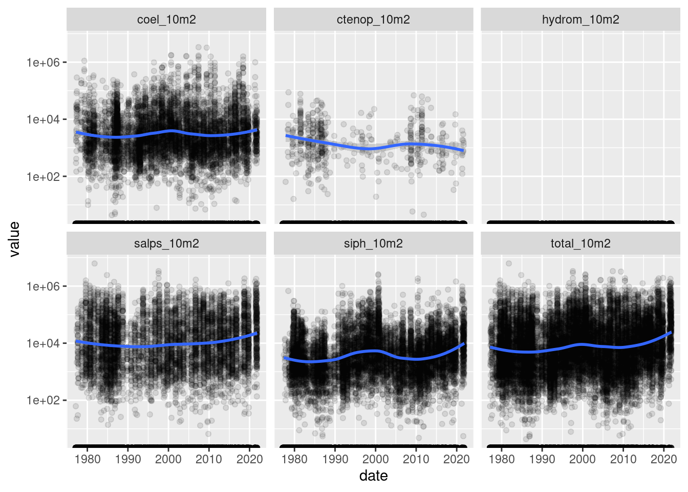
$ value <dbl> 0.00, 0.00, 27667.03, 0.00, 0.00, 27667.03, 0.00, 0.00, 0.…ggplot(data = long,
mapping = aes(x = date, y = value)) +
geom_point(alpha = 0.1) +
geom_smooth(method = "loess", formula = "y~x") +
scale_y_continuous(trans='log10') +
facet_wrap(~name)
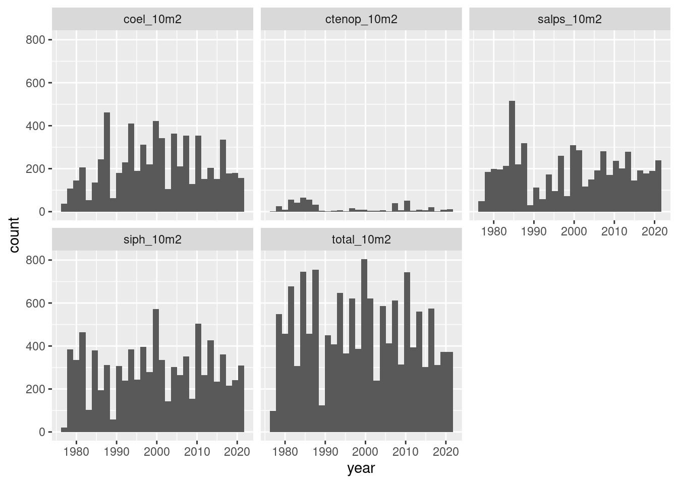
Let’s look at coverage by year - note we are counting occurences (absences dropped) which results in the exclusion of Hydromedusea.
long = mutate(long, year = as.numeric(format(date, "%Y")),
              month = as.numeric(format(date, "%m")))

ggplot(data = filter(long, value > 0),
       mapping = aes(year)) +
  geom_histogram() +
  facet_wrap(~name)
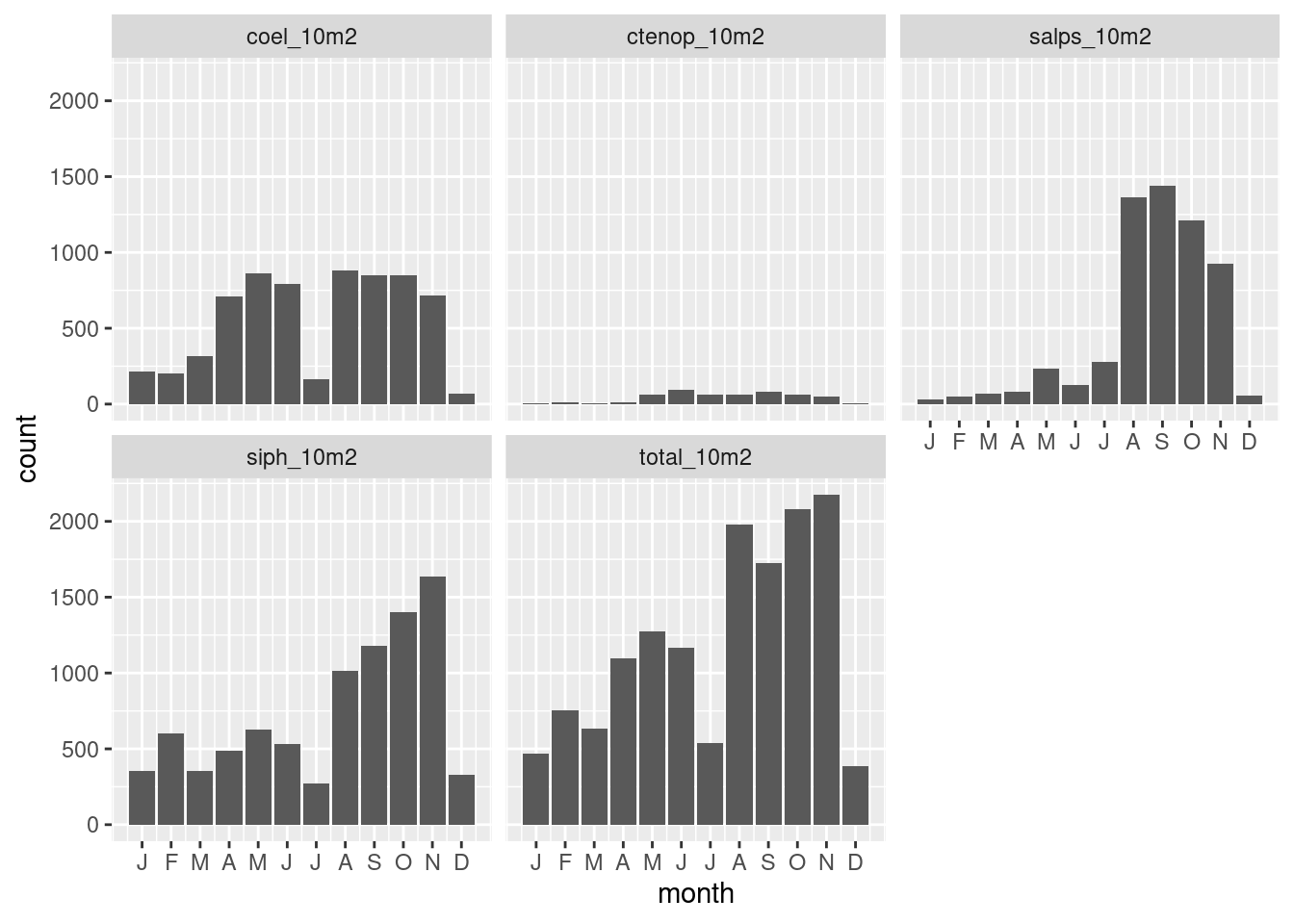
And alternative is to look at the observations by month.
ggplot(data = filter(long, value > 0),
       mapping = aes(month)) +
  geom_histogram(stat = "count") +
  scale_x_continuous(breaks = 1:12,
                     labels = function(x) substring(month.abb[x],1,1)) +
  facet_wrap(~name)
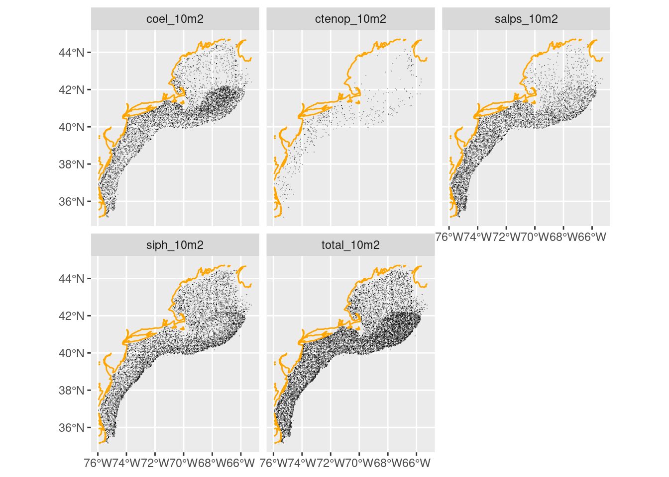
We can read the same data in a spatial form and plot that. Once again, we exclude sample locations where there are absences.
long = ecomon_as_sf(filter(long, value > 0))
coast = ne_coastline(scale = "medium", returnclass = "sf") |>
  st_crop(long)

ggplot() +
  geom_sf(data = long, shape = ".", alpha = 0.3) +
  geom_sf(data = coast, color = "orange") +
  facet_wrap(~name)