here() starts at /mnt/s1/projects/ecocast/projects/jellyscapeSalpsae
thisgroup = "Salps"
x = read_ecomon_spp(form = 'sf', groups = thisgroup, agg = FALSE) |>
  ecomon_to_long() |>
  dplyr::mutate(year = format(date, "%Y") ,
                month = factor(format(date, "%b"), levels = month.abb))
nonz = dplyr::filter(x, value > 0)
zero = dplyr::filter(x, value <= 0)
n = nrow(x)
nz = zero |> nrow()
coast = sf::st_crop(coast, x)
There are 32693 records for salps of which 23202 are zeroes (about 70.97%) leaving 9491 non-zero salp abundance records.
1 Non-zero abundances
Here’s an abudnance scaled plot of the non-zero abundances.
Code
plot(nonz['value'],
     pch = ".",
     logz = TRUE,
     main = glue::glue("Non-zero abundance of {thisgroup}"),
     axes = TRUE,
     reset = FALSE)
plot(coast, add = TRUE, col = "black")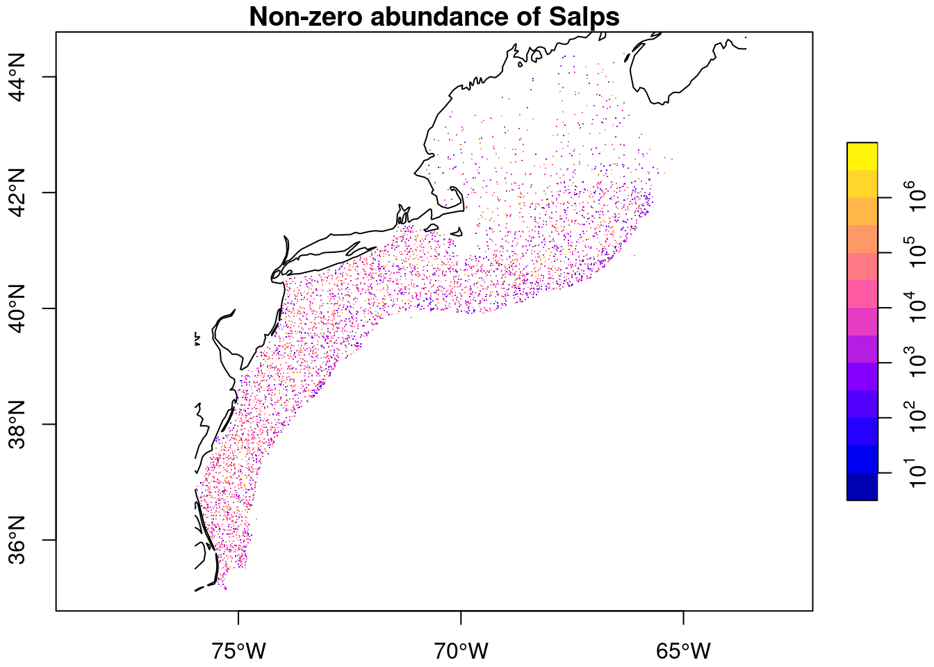
Code
ggplot(data = dplyr::group_by(nonz, year),
       mapping = aes(x = year)) +
  geom_bar() +
  theme(axis.text.x = element_text(angle = 90, vjust = 0.5, hjust=1)) +
  labs(y = "Record count", title = glue::glue("Non-zero abundance {thisgroup} Records by Year"))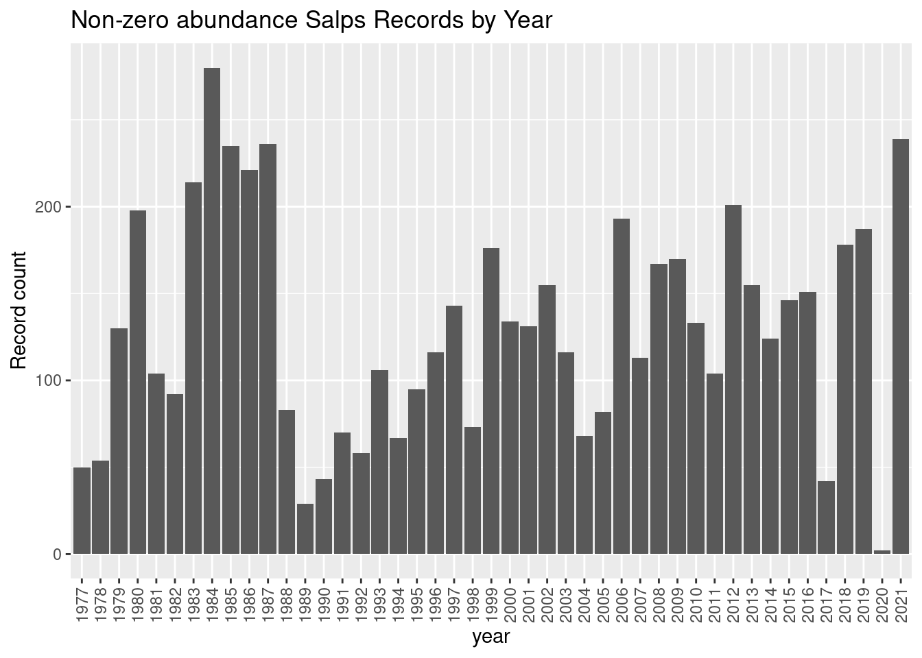
Code
ggplot(data = dplyr::group_by(nonz, month),
       mapping = aes(x = month)) +
  geom_bar() +
  theme(axis.text.x = element_text(angle = 90, vjust = 0.5, hjust=1)) +
  labs(y = "Record count", title = glue::glue("Non-zero abundance {thisgroup} Records by Month"))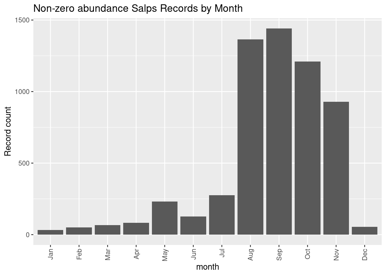
2 Zero Abundance (i.e. absences)
The distribution of zero abundance records is much more extensive.
Code
plot(zero['value'] |>
       dplyr::filter(value <= 0) |>
       sf::st_geometry(),
     pch = ".",
     main = glue::glue("Zero abundance presences {thisgroup}"),
     axes = TRUE,
     reset = FALSE)
plot(coast, add = TRUE, col = "black")
Code
ggplot(data = dplyr::group_by(zero, year),
       mapping = aes(x = year)) +
  geom_bar() +
  theme(axis.text.x = element_text(angle = 90, vjust = 0.5, hjust=1)) +
  labs(y = "Record count", title = glue::glue("Zero abundance {thisgroup} Records by Year"))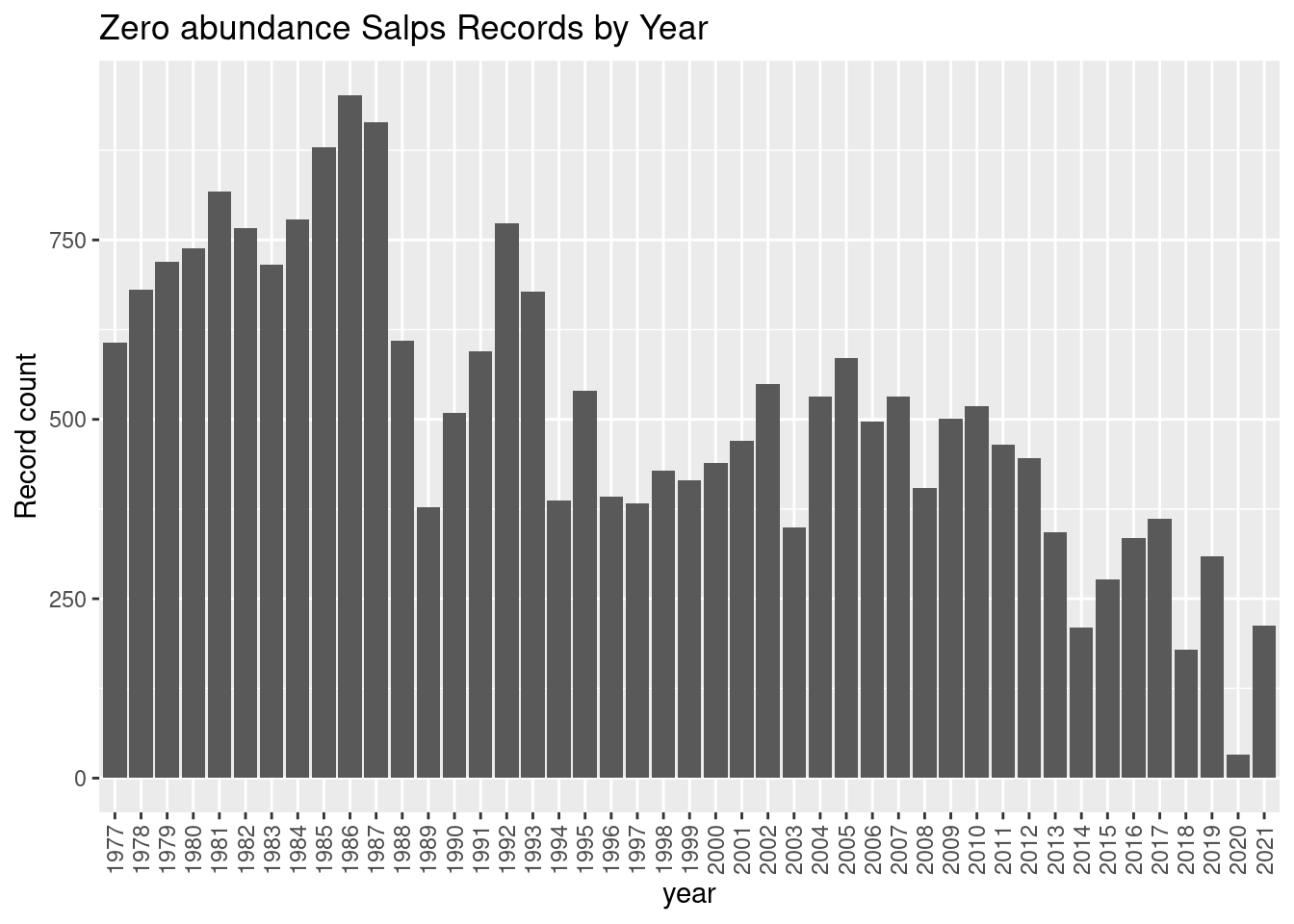
Code
ggplot(data = dplyr::group_by(zero, month),
       mapping = aes(x = month)) +
  geom_bar() +
  theme(axis.text.x = element_text(angle = 90, vjust = 0.5, hjust=1)) +
  labs(y = "Record count", title = glue::glue("Zero abudnance {thisgroup} Records by Month"))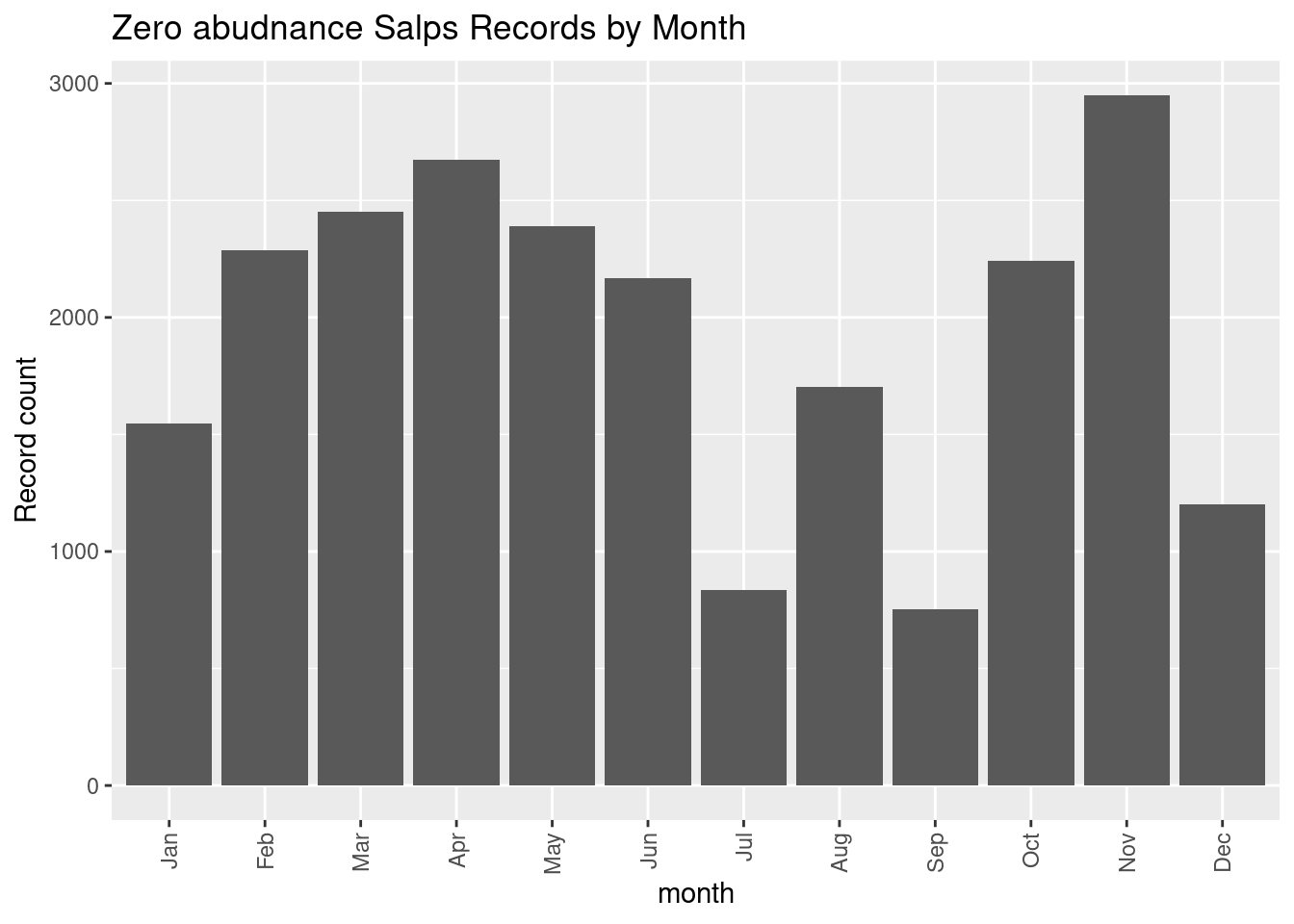
3 A closer look at non-zero abundances
We can bin the data into abundance quantiles.
quants = seq(from = 0, to = 0.95, by = 0.05)
qs = quantile(nonz$value, quants)
ix = findInterval(nonz$value, qs)
nonz = dplyr::mutate(nonz,
                     quantile = quants[ix],
                     percentile = factor(names(qs)[ix], levels = names(qs)))
Code
ggplot(data = nonz) +
  geom_sf(alpha = 0.1, size = 0.3) +
  geom_sf(data = coast,
          color = "orange") +
  facet_wrap(~percentile)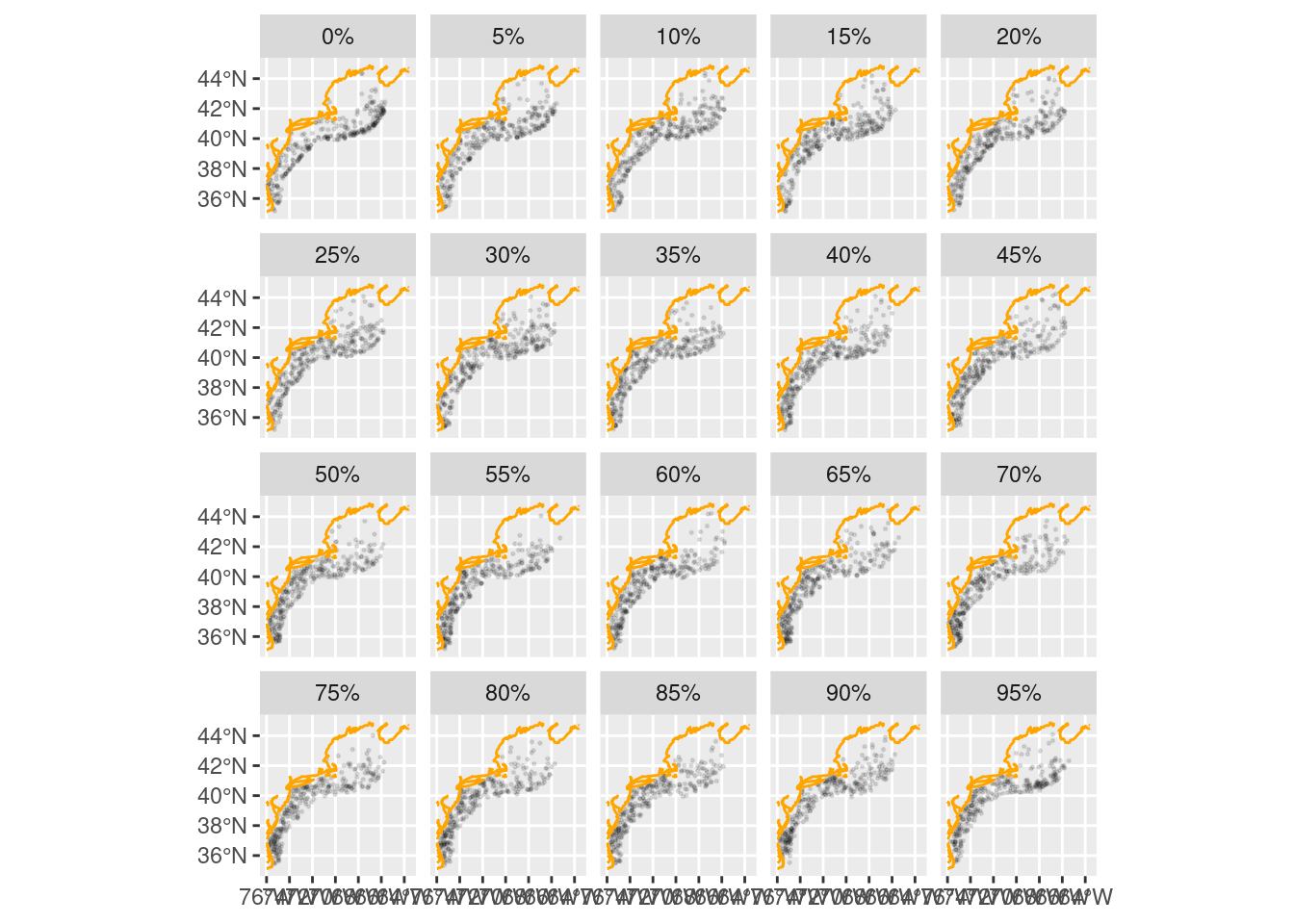
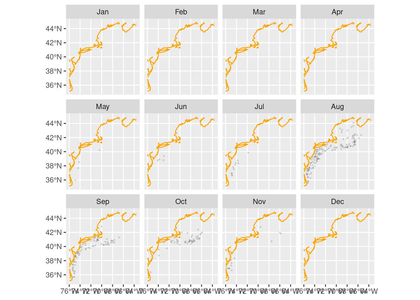
4 A closer look at the top 5% abundances
Code
top5 = dplyr::filter(nonz, quantile >= 0.95)

ggplot(data = top5) +
  geom_sf(alpha = 0.1, size = 0.4) +
  geom_sf(data = coast,
          color = "orange") +
  facet_wrap(~month, drop = FALSE)