Here we do the multi-step task of associating observations with environmental covariates and creating a background point data set used by the model to characterize the environment.
1 Background points to characterize the environment
Presence only modeling using MaxEnt or the pure R implementation maxnet require that a sample representing “background” is provided for the model building stage. Background points are used to characterize the environment in which the presence points are found, the modeling algorithm uses that information to discriminate between suitability and unsuitability of the environment. It is good practice to sample “background” in the same spatial and temporal range as the presence data. That means we need to define a bounding polygon around the presence locations from which we can sample, as well as sampling through time.
2 Loading data
We have two data sources to load: point observation data and rasterized environmental predictor data.
2.1 Load the observation data
We’ll load in our OBIS observations as a flat table, and immediately filter the data to any occurring from 2000 to present.
Next we load the environmental predictors, sst and wind (as windspeed, u_wind and v_wind). For each we first read in the database, then call a convenience reading function that handles the input of the files and assembling into a single stars class object.
stars object with 3 dimensions and 4 attributes
attribute(s):
                 Min.   1st Qu.       Median        Mean   3rd Qu.      Max.
sst         -1.605714 13.091935 19.337191582 17.76428969 23.201612 30.208710
windspeed    0.000000  6.530073  8.142477036  8.24075914  9.938321 16.516525
u_wind      -5.537110  1.101731  2.489401579  2.68725622  4.097867 13.148120
v_wind     -15.890004 -1.264965  0.007917786  0.01049414  1.277609  9.274651
             NA's
sst        233700
windspeed  179169
u_wind     179169
v_wind     179169
dimension(s):
     from  to offset delta refsys point                    values x/y
x       1  74 -76.38  0.25 WGS 84 FALSE                      NULL [x]
y       1  46  46.12 -0.25 WGS 84 FALSE                      NULL [y]
time    1 285     NA    NA   Date    NA 2000-01-01,...,2023-09-01
We’ll set these aside for a moment and come back to them after we have established our background points.
3 Sampling background data
We need to create a random sample of background in both time and space.
3.0.1 How many samples?
Now we can sample - but how many? Let’s start by selecting approximately four times as many background points as we have observation points. If it is too many then we can sub-sample as needed, if it isn’t enough we can come back an increase the number. In addition, we may lose some samples in the subsequent steps making a spatial sample.
3.1 Sampling time
Sampling time requires us to consider that the occurrences are not evenly distributed through time. We can see that using a histogram of observation dates by month.
First, let’s add a variable to obs that reflects the first day of the month of the observation. We’ll use the current_month() function from the oisster package to compute that. We then use that to define the breaks (or bins) of a histogram.
obs = obs |> dplyr::mutate(month_id = oisster::current_month(date))date_range =range(obs$month_id)breaks =seq(from = date_range[1], to = date_range[2], by ="month")H =hist(obs$month_id, breaks = breaks, format ="%Y", freq =TRUE, main ="Observations",xlab ="Date")
Clearly the observations bunch up during certain times of the year, so they are not randomly distributed in time.
Now we have a choice… sample randomly across the entire time span or weight the sampling to match that the distribution of observations. Context matters. Since observations are not the product of systematic surveys, but instead are presence observations we need to keep in mind we are modeling human behavior: we are modeling observations of people who report observations.
3.1.1 Unweighted sampling in time
If the purpose of the sampling isn’t to mimic the distribution of observations in time, but instead to characterize the environment then we would make an unweighted sample across the time range.
Note
Note that we set the random number generator seed. This isn’t a requirement, but we use it here so that we get the same random selection each time we render the page. Here’s a nice discussion about set.seed()usage.
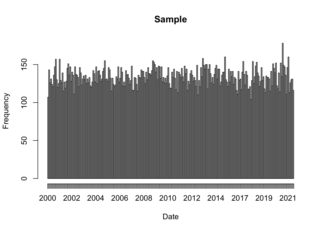
Now we can plot the same histogram, but with the days_unweighted_sample data.
unweightedH =hist(days_sample, breaks ='month', format ="%Y", freq =TRUE, main ="Sample",xlab ="Date")
3.1.2 Weighted sampling in time
Let’s take a look at the same process but this time we’ll use a weight to sample more when we tend to have more observations. We’ll use the original histogram counts
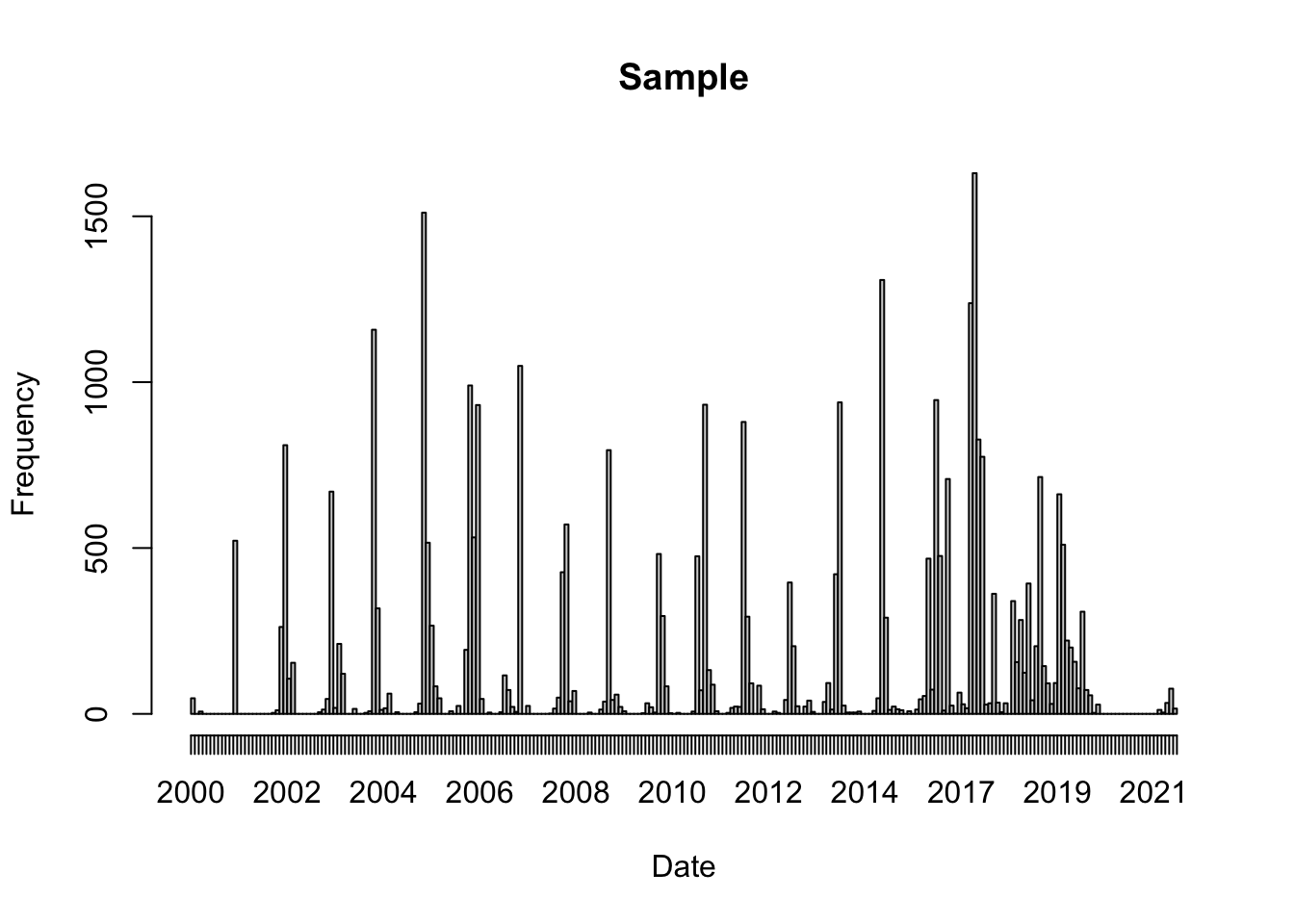
Now we can plot the same histogram, but with the days_unweighted_sample data.
weightedH =hist(days_sample, breaks ='month', format ="%Y", freq =TRUE, main ="Sample",xlab ="Date")
In this case, we are modeling the event that an observer spots and reports a Mola mola, so we want to background to characterize the times when those events occur. We’ll use the weighted time sample.
3.2 Sampling space
The sf package provides a function, st_sample(), for sampling points within a polygon. But what polygon? We have choices as we could use (a) a bounding box around the observations, (b) a convex hull around the observations or (c) a buffered envelope around the observations. Each has it’s advantages and disadvantages. We show how to make one of each.
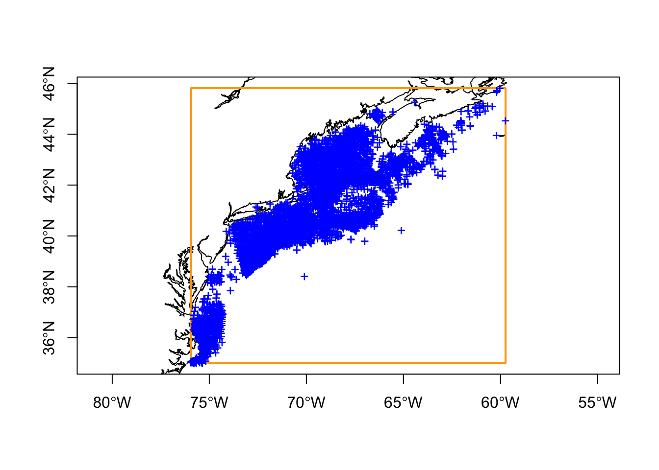
3.2.1 The bounding box polygon
This is the easiest of the three polygons to make.
Hmmm. It is easy to make, but you can see vast stretches of sampling area where no observations have been reported (including on land). That could limit the utility of the model.
3.2.2 The convex hull polygon
Also an easy polygon to make is a convex hull - this is one often described as the rubber-band stretched around the point locations. The key here is to take the union of the points first which creates a single MULTIPOINT object. If you don’t you’ll get a convex hull around every point… oops.
Well, that’s an improvement, but we still get large areas vacant of observations and most of Nova Scotia.
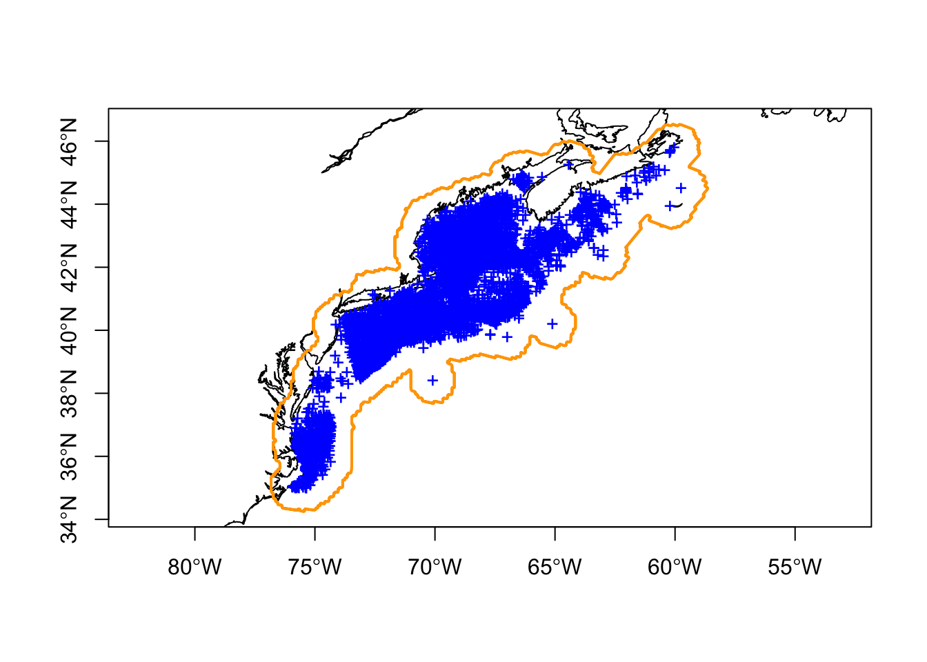
3.2.3 The buffered polygon
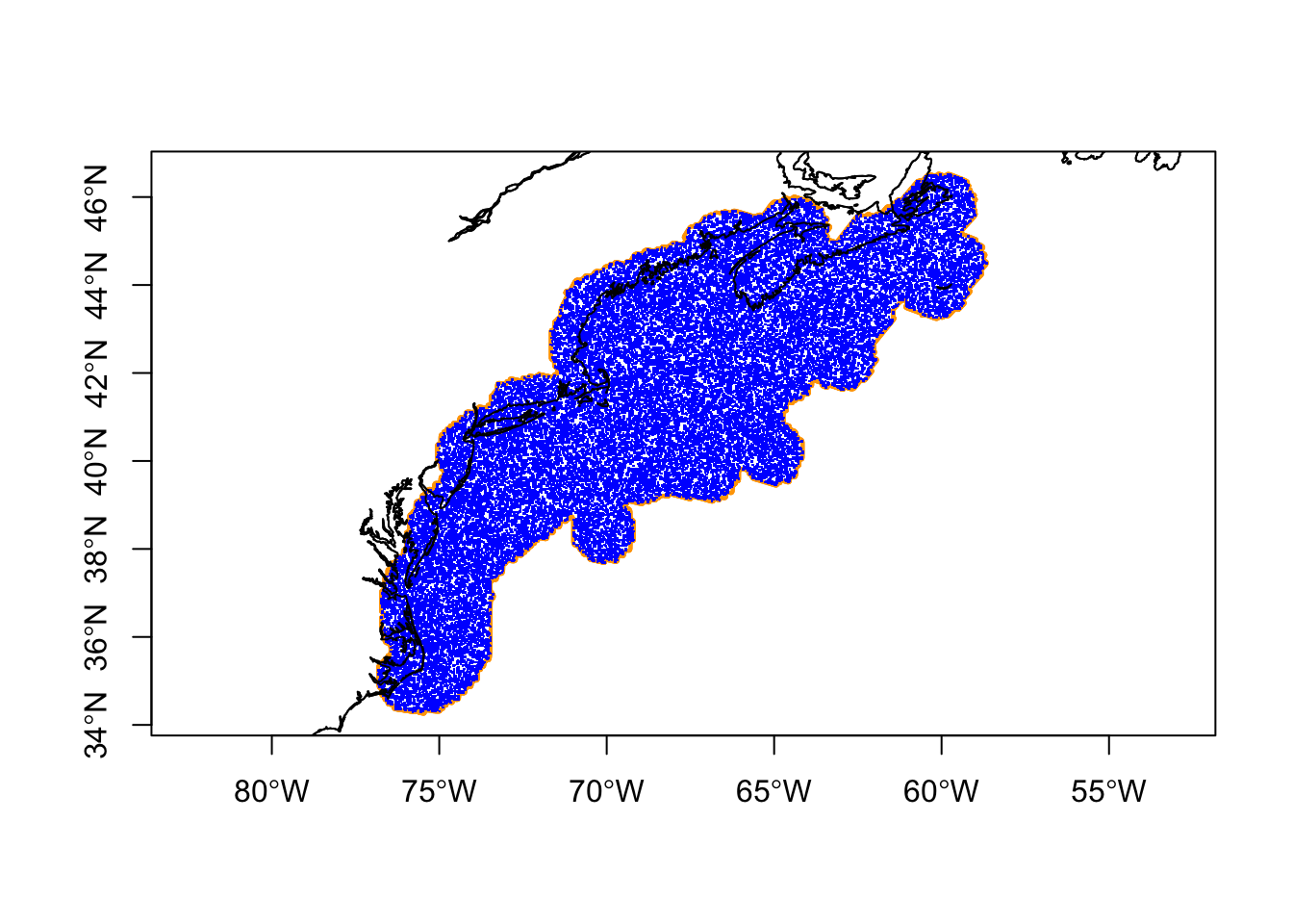
An alternative is to create a buffered polygon around the MULTIPOINT object. We like to think of this as the “shrink-wrap” version as it follows the general contours of the points. We arrived at a buffereing distance of 75000m through trial and error, and the add in a smoothing for no other reason to improve aesthetics.
That seems the best yet, but we still sample on land. We’ll over sample and toss out the ones on land. Let’s save this polygon in case we need it later.
ok =dir.create("data/bkg", recursive =TRUE, showWarnings =FALSE)sf::write_sf(poly, file.path("data", "bkg", "buffered-polygon.gpkg"))
3.2.4 Sampling the polygon
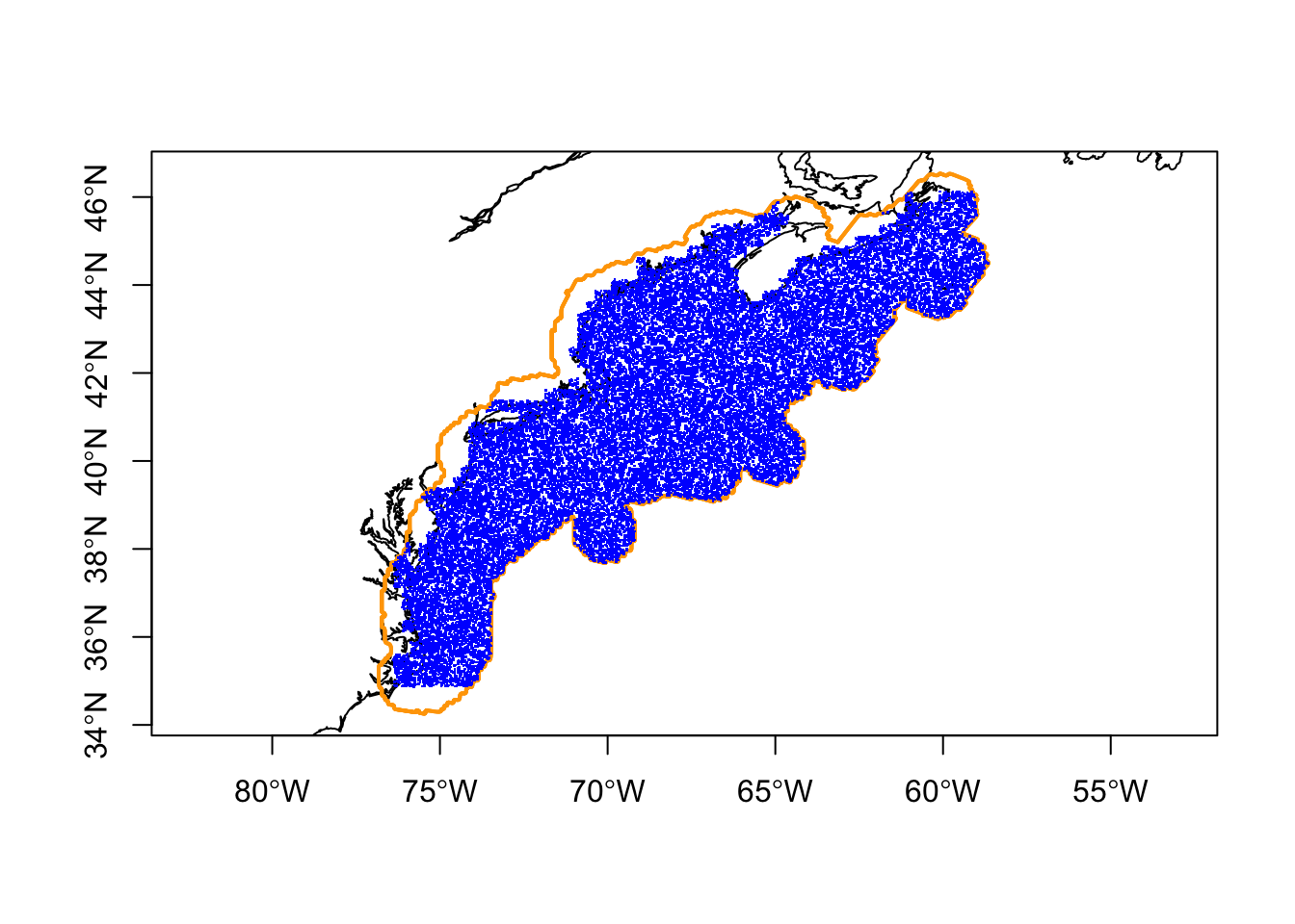
Now to sample the within the polygon, we’ll sample the same number we selected earlier. Note that we also set the same seed (for demonstration purposes).
OK - we can work with that! We still have points on land, but most are not. The following section shows how to use SST maps to filter out errant background points.
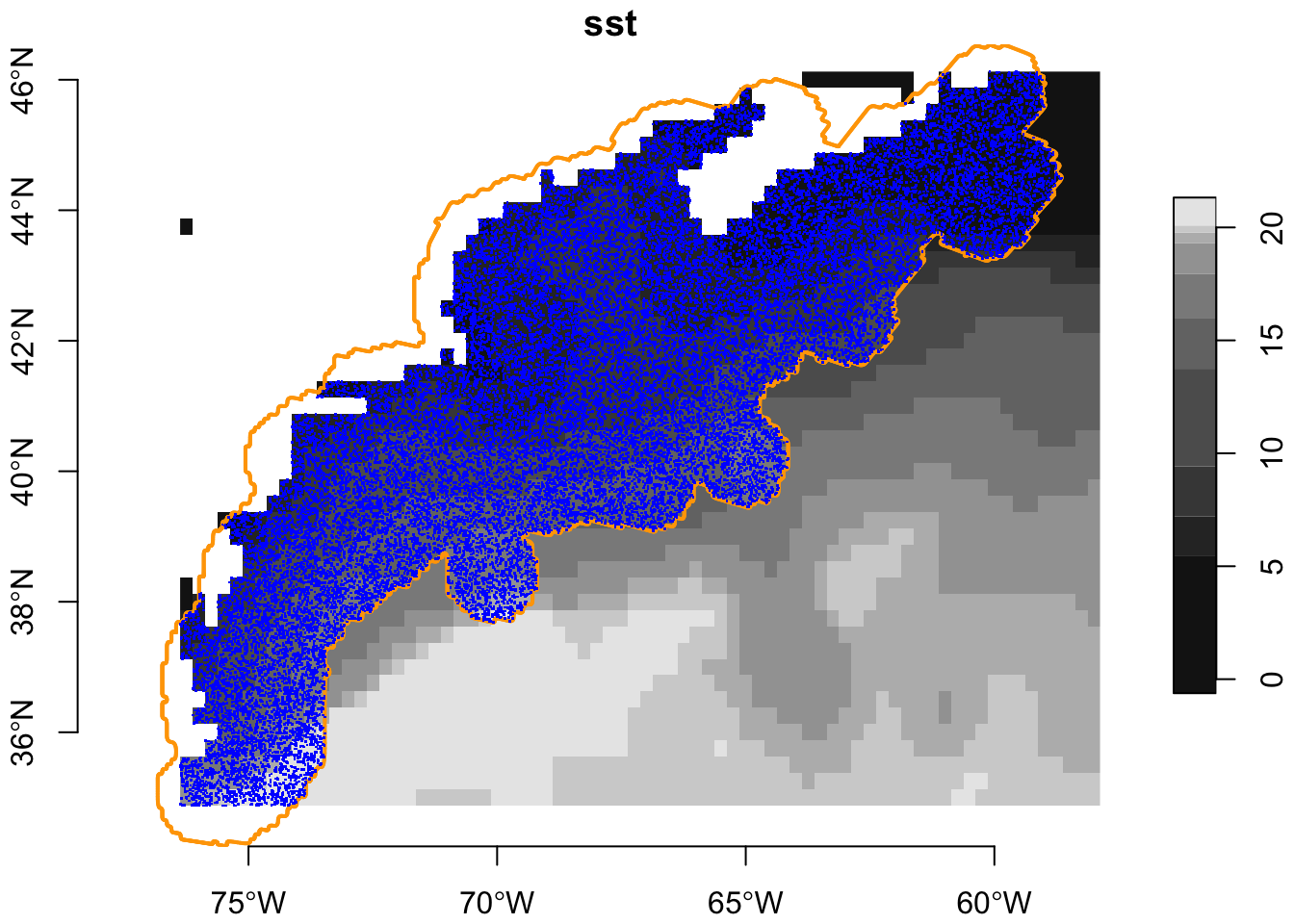
3.2.5 Purging points that are on land (or very nearshore)
It’s great if you have in hand a map the distinguishes between land and sea - like we do with sst. We shall extract values v from just the first sst layer (hence the slice).
Values where sst are NA are beyond the scope of data present in the OISST data set, so we will take that to mean NA is land (or very nearshore). We’ll merge our bkg object and random dates (days_sample), filter to include only water.
4 Extract environmental covariates for sst and wind
4.1 Wait, what about dates?
You may have considered already an issue connecting our background points which have daily dates with our covariates which are monthly (identified by the first of each month.) We can manage that by adding a second date, month_id, to the bkg table.
Here we go back to the complete covariate dataset, preds. We extract specifying which variable in bkg is mapped to the time domain in sst - in our case the newly computed month_id matches the time dimension in sst. We’ll save the values while we are at it.
It’s the same workflow to extract covariates for the observations as it was for the background, but let’s not forget to add in a variable to identify the month that matches those in the predictors.