source("setup.R")Background
No choice is the wrong choice as long as you make a choice. The only wrong choice is choosing not to make one. ~ Jake Abel
Traditional ecological surveys are systematic, for a given species survey data sets tell us where the species is found and where it is absent. Using an observational data set (like OBIS) we only know where the species is found, which leaves us guessing about where they might not be found. This difference is what distinguishes a presence-abscence data set from a presence-only data set, and this difference guides the modeling process.
When we model species distributions we are trying to define the environments where we should expect to find a species as well as the environments we would not expect to find a species. With OBIS data we have in hand the locations of observations, and we can extract the environmental data at those locations. To characterize the unoccupied environments we are going to have to sample what is called “background” (aka “background points” and “pseudo-absences”.)
We assume that we want the number of background points to be roughoy balanced with the number of observations. What balance means is open to interpretation, but if we have 100 observations then we would like to have 50 to 200 background points in order to be balanced. One can spend a lot of time of time finding the most appropriate balance.
We want these background samples to roughly match the regional preferences of the observations; that is we want to avoid having observations that are mostly over Georges Bank while our background samples are primarily around the Bay of Fundy. We want there to be some reasonable proximity between occupied and unoccupied environments.
Here we want to satisfy a couple of basic requirements…
balance the number of observations and background points (whatever balance means),
avoid selecting background points that coincide with observations,
choose background points where we can measure the same environmental characteristics that we can measure for observations.
Keep in mind we will be glossing over important details; there is much more to investigate here, but tempus fugit and our course of study is brief. At the end we want to have in hand a set of locations that can be a companion for the observations.
1 Setup
As always, we start by running our setup function. Start RStudio/R, and relaod your project with the menu File > Recent Projects.
We also will need the Brickman mask and the observation data. Note that we are making a model that works for every month, so we shall select background points by month. Given what we have learned about the distribution of observations over the months of year this may be surprising; some months have many more observations than other months. Won’t months with more data be “better informed” than months with fewer data? That is possible, but we have to start somewhere so we’ll be choosing a set number of background points for each month that balances the observations and background throughout the year rather than per month.
OK - load the data we need.
coast = read_coastline()
obs = read_observations(scientificname = "Mola mola")
db = brickman_database() |>
  filter(scenario == "STATIC", var == "mask")
mask = read_brickman(db)
Let’s start with a simple plot of the observations per month. We’ll make an array of maps with one constructed per month. We’ll use the ggplot2 plotting system which is a powerful system for layering components of a plot.
We will want to add a notation to each plot showing the number of points that month. To make that table we use the count() function from the dplyr R package. We also found the best location to print the count (through trial and error) so we define that, too.
LON0 = -67
LAT0 = 46
all_counts = count(st_drop_geometry(obs), month) # counting is faster without spatial baggage
all_counts
# A tibble: 12 × 2
month n
<fct> <int>
1 Jan 5
2 Feb 17
3 Mar 14
4 Apr 247
5 May 670
6 Jun 2347
7 Jul 2086
8 Aug 2520
9 Sep 929
10 Oct 426
11 Nov 338
12 Dec 56Now we can construct the plot. Note that layering of data, then the coast then the extra text. Also, we use alpha (aka ‘transparency’ or ‘opacity’) blending to make the plotting symbols slightly transparent which reveals overlapping points nicely.
ggplot() +
  geom_sf(data = obs, alpha = 0.2, shape = "circle small", size = 1) +
  geom_sf(data = coast, col = "orange") +
  geom_text(data = all_counts,
            mapping = aes(x = LON0,
                          y = LAT0,
                          label = sprintf("n: %i", .data$n)),
                          size = 3) +
  labs(x = "Longitude", y = "Latitude", title = "All observations") +
  facet_wrap(~month)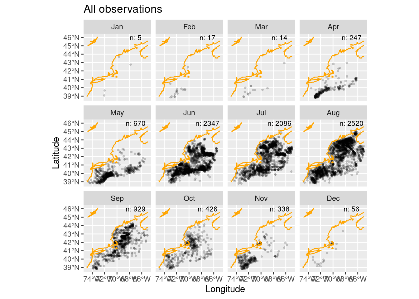
Some of those points are densely distributed depending upon the month. In fact, it may be that we have multiple points in each raster cell in our Brickman data. We have a function to help use reduce “thin” the observations so that we have just one observation per cell.
1.1 Thinning observations
Thinning is the process we use to sub-sample observations so that they are more evenly sampled across the spatial domain. We do this to discourage accidental sampling bias. The tidysdm package provides a nice function, thin_by_cell(), that “thins” by allowing only one observation per cell in the Brickman data. We’ll iterate through each month
thinned_obs = sapply(month.abb,
               function(mon){
                 thin_by_cell(obs |> filter(month == mon), mask)
               }, simplify = FALSE) |>
  dplyr::bind_rows()

# another count
thinned_counts = count(st_drop_geometry(thinned_obs), month)

ggplot() +
  geom_sf(data = thinned_obs,
          alpha = 0.2,
          shape = "circle small",
          size = 1) +
  geom_sf(data = coast, col = "orange") +
  geom_text(data = thinned_counts,
            mapping = aes(x = LON0,
                          y = LAT0,
                          label = sprintf("n: %i", .data$n)),
                          size = 3) +
  labs(x = "Longitude", y = "Latitude", title = "Thinned observations") +
  facet_wrap(~month)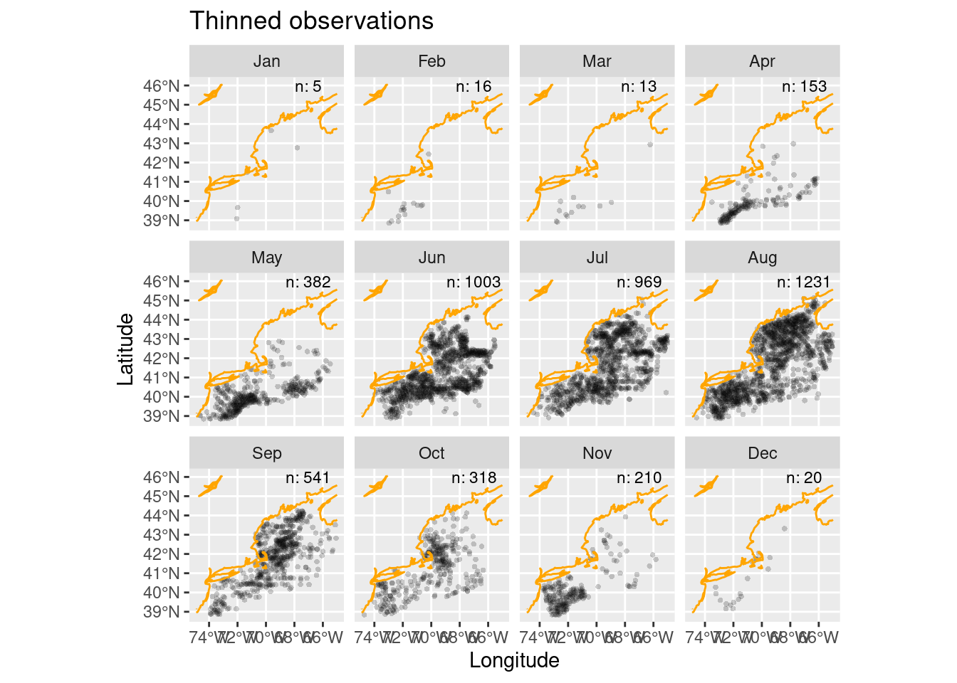
1.2 Weighted sampling
We now have thinned the observations to just 4861 records compared to the original 9655 observations. So that get us to no more than 1 observation to cell. But do we loose the importance of clustered observations? Isn’t meaningful ecologically that the species is found in clusters? The answers to those are yes and yes.
Uh oh, so how do we retain that clustering importance? The answer is to build a sampling bias map using the original observations that influences where we sample. Let’s build a bias map by counting the number of observations in each cell - we’ll use the original observations for the entire year (regardless of month.)
bias_map = rasterize_point_density(obs, mask) # <-- note the original observations

ggplot() +
  geom_stars(data = bias_map, aes(fill = count)) +
  scale_fill_viridis_b(na.value = "transparent") +
  geom_sf(data = coast, col = "orange") +
  labs(x = "Longitude", y = "Latitude", title = "Bias map using all observations")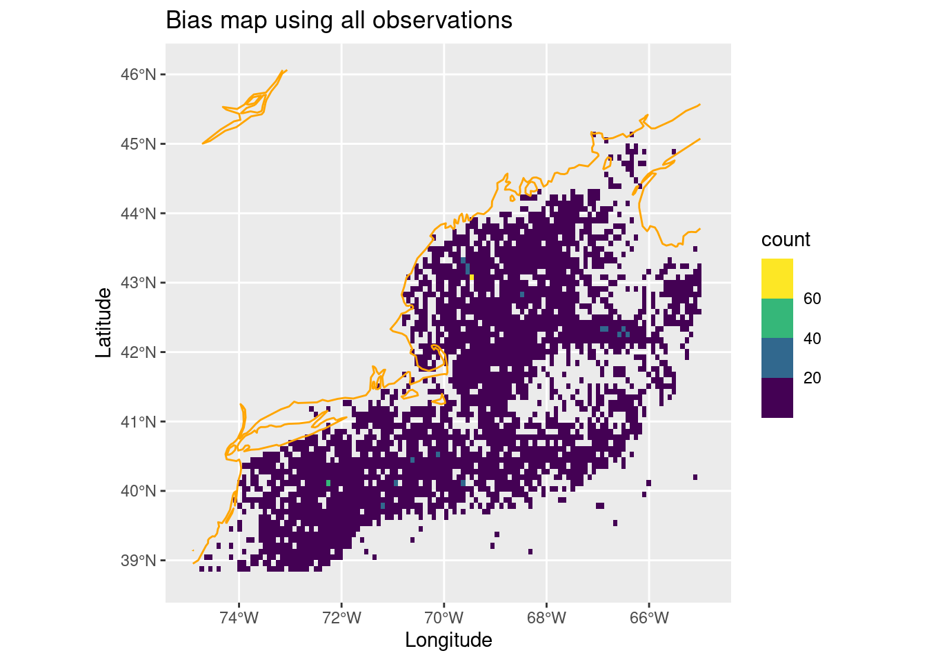
Depending upon your distribution, the clustering may be more or less apparent. For Mola mola it’s dominated by a wide even spread with a few “peak” spots.
1.3 Randomly sample background points
Now that we have a reasonable set of observation and a sampling bias map, we now need to choose points using those to represent the background. The sample_background() function requires three input arguments: the set of observations, the raster array and the number of points desired. We can also ask for the presence observations to be returned along with the background points to keep things tidy. Since we are doing this by month, we’ll modify the output by adding a column identifying the month.
1.3.0.1 But just how many background points?
But how many background points should we get for each month? Should be try balance by month? Or balance by taking the average for all months. Let’s do the latter, but it might be worth exploring that further.
nback_avg = mean(all_counts$n) |>
  round()
nback_avg
[1] 805So, here we go. We shall use the sapply iterator to step through each month. For each month we’ll use the thinned observations and the annual bias map to sample for background. At the end we’ll have a list of monthly tables which we’ll bind into one giant table, and we’ll refresh the month column to be a factor (of monthly groupings of course!)
obsbkg = sapply(month.abb,
    function(mon){
      sample_background(thinned_obs |> filter(month == mon), # <- just this month
                       bias_map,
                       method = "bias",  # <-- it needs to know it's a bias map
                       return_pres = TRUE, # <-- give me the obs back, too
                       n = nback_avg) |>   # <-- how many points
        mutate(month = mon, .before = 1)
    }, simplify = FALSE) |>
  bind_rows() |>
  mutate(month = factor(month, levels = month.abb))
obsbkg
Simple feature collection with 14521 features and 2 fields
Geometry type: POINT
Dimension: XY
Bounding box: xmin: -74.72716 ymin: 38.84118 xmax: -65.00391 ymax: 45.1333
Geodetic CRS: WGS 84
# A tibble: 14,521 × 3
month class geometry
* <fct> <fct> <POINT [°]>
1 Jan presence (-71.989 39.668)
2 Jan presence (-69.62994 43.65584)
3 Jan presence (-67.79617 42.75941)
4 Jan presence (-71.31 41.49)
5 Jan presence (-72.05151 39.07928)
6 Jan background (-66.50078 42.33478)
7 Jan background (-72.5883 40.44271)
8 Jan background (-69.21549 41.5944)
9 Jan background (-72.91736 39.37328)
10 Jan background (-69.05096 39.7846)
# ℹ 14,511 more rowsA quick tally of the class by month confirms that our nback_avg of 805 points is used consistently every month.
# drop the spatial baggage to speed the tally
count(st_drop_geometry(obsbkg), month, class)
# A tibble: 24 × 3
month class n
<fct> <fct> <int>
1 Jan presence 5
2 Jan background 805
3 Feb presence 16
4 Feb background 805
5 Mar presence 13
6 Mar background 805
7 Apr presence 153
8 Apr background 805
9 May presence 382
10 May background 805
# ℹ 14 more rowsLet’s see where these presence/background points fall relative to each other.
ggplot() +
  geom_sf(data = obsbkg,
          mapping = aes(col = class),
          alpha =  0.4, shape = "circle small", size = 1) +
  geom_sf(data = coast, col = "orange")  +
  labs(x = "Longitude", y = "Latitude", title = "All") +
  theme_bw() +  # <- make a simple white background
  scale_fill_okabe_ito() +  # <-- colorblind friendly for N Record
  facet_wrap(~month)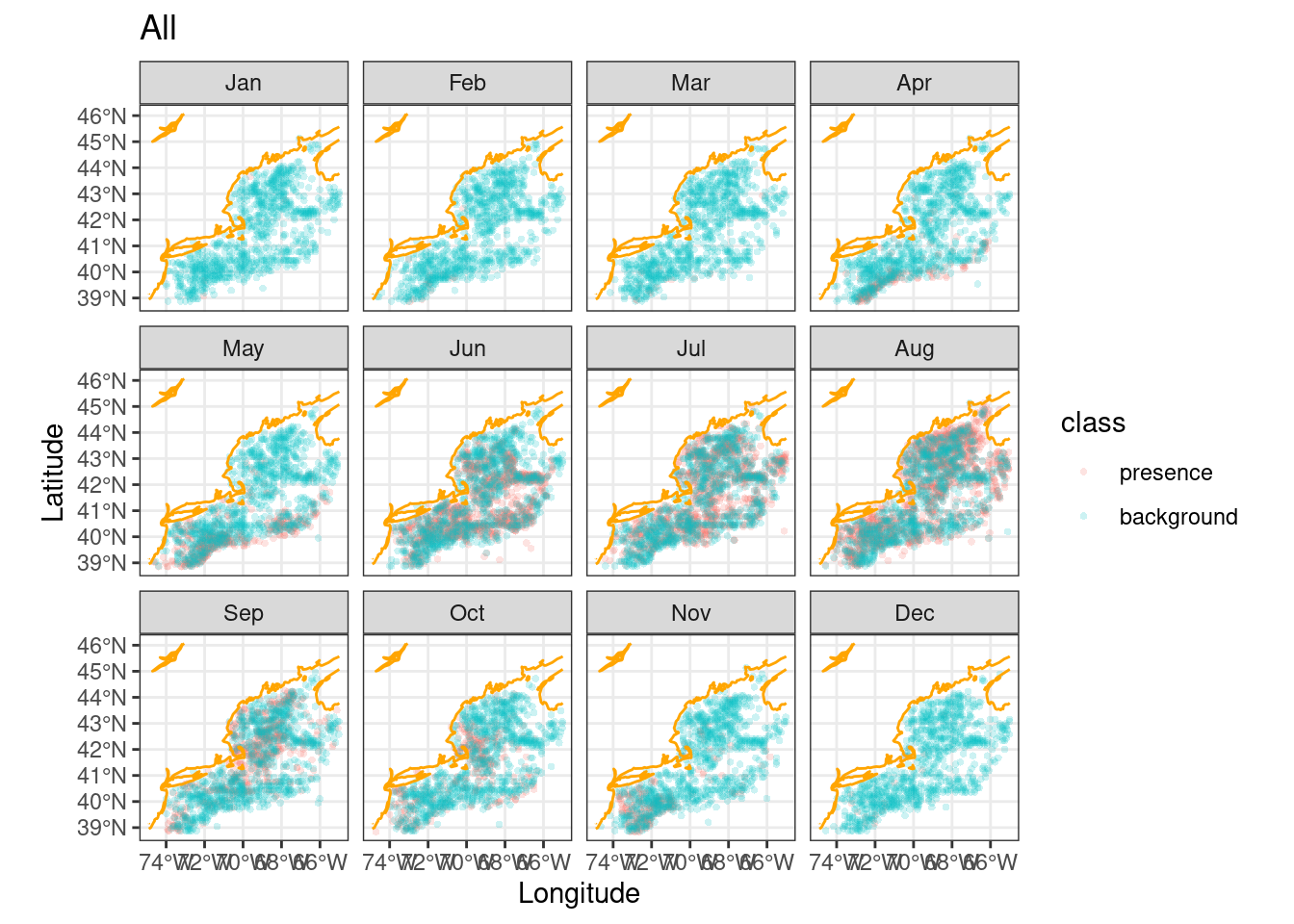
These would be the data locations we feed into the model. So is that reasonable solution? At first glance it seems to be, so we’ll choose this background sampling approach; thinning with biased sampling. We can’t know if another approach might be better until we actually start modeling.
Let’s save this.
write_model_input(obsbkg, scientificname = "Mola mola")Note that there is a function for reading model input files, too.
x = read_model_input(scientificname = "Mola mola")2 Recap
We have prepared what we call “model inputs”, in particular for Mola mola, by thinning observations and selecting background points. There are lots of other approaches to creating the model input, but for the sake of learning we’ll stick with this approach. We developed a function that will produce our model inputs for a given month, and saved them to disk.
3 Coding Assignment
Use the menu option File > New File > R Script to create a blank file. Save the file (even though it is empty) in the “assignment” directory as “assignment_script_2.R”. Use this file to build a script that meets the following challenge. Note that the existing file, “assignment_script_0.R” is already there as an example.
For each month select at random one presence and one background point (so, that will be 2 x 12 = 24 points!) from your model input data. Then select three (3) variables in the Brickman present monthly data set, and build a single table that has the three variables for the 24 points. This is very similar to the C00 coding chapter homework.
Hint! Check out iterating over grouped tables and the slice_sample function.
Here’s what our table looks like for the Mola mola species.
Simple feature collection with 24 features and 7 fields
Geometry type: POINT
Dimension:     XY
Bounding box:  xmin: -72.99962 ymin: 39.07928 xmax: -65.51362 ymax: 43.89779
Geodetic CRS:  WGS 84
# A tibble: 24 × 8
   month class                      geom point  depth   SSS   SST  Tbtm
 * <fct> <fct>               <POINT [°]> <chr>  <dbl> <dbl> <dbl> <dbl>
 1 Jan   presence   (-72.05151 39.07928) p1    2116.   33.3 10.9   3.72
 2 Jan   background (-67.48795 40.36045) p2     789.   31.7  6.65  4.67
 3 Feb   presence   (-72.00363 39.67702) p1     231.   31.9  5.73  8.64
 4 Feb   background (-69.79134 40.60724) p2      60.4  31.2  3.58  3.89
 5 Mar   presence       (-72.056 39.205) p1    1362.   32.4  6.98  4.13
 6 Mar   background (-67.73474 42.66383) p2     194.   30.9  1.88  7.58
 7 Apr   presence      (-72.263 39.4379) p1     386.   31.7  7.08  6.44
 8 Apr   background  (-72.8351 39.20875) p2     102.   31.5  6.74 10.3
 9 May   presence          (-66.3 41.25) p1     281.   31.2  8.03  7.12
10 May   background (-71.43661 39.62007) p2    1867.   31.9 11.4   3.78
# ℹ 14 more rows
# ℹ Use `print(n = ...)` to see more rows