source("setup.R")Covariates
- “In the end that was the choice you made, and it doesn’t matter how hard it was to make it. It matters that you did.”
- Cassandra Clare
Now we turn our attention to what we know and guess about the environments. We are using the Brickman data to make habitat suitability maps for select species under two climate scenarios (RCP45 and RCP85) at two different times (2055 and 2075) in the future. Each variable we might use is called a covariate or predictor. Our covariates are nicely packaged up and tidy, but the reality is that it often requires a good deal of data wrangling if the data are messy.
Our step here is to make sure that two or more covariates are not highly correlated if they are, then we would likely want to drop all but one. This comes with a caveat though… as marine ecologists we know that water depth is always important, and we know that time of year (in our case month) is always important. So, regardless of what our analyses of covariates may tell us, we are going to make darn sure that depth and month are included.
1 Setup
As always, we start by running our setup function. Start RStudio/R, and reload your project with the menu File > Recent Projects.
2 A broad approach - looking for correlation across the domain
We can look at the entire domain, the complete spatial extent of our arrays of data, to look for correlated variables. For example, we might wonder if sea surface temperature (SST) and sea floor temperature (Tbtm) vary together, that is when one goes up does the other goes up? That sort of thing. We have ways of getting at those correlations.
2.1 Reading in the covariates
We’ll read in the Brickman database, then filter two different subsets to read: “STATIC” covariate bathymetry that apply across all scenarios and times and monthly covariates for the “PRESENT” period.
db = brickman_database() |>
  dplyr::filter(scenario == "PRESENT", interval == "mon")
present = read_brickman(db)
2.2 Make a pairs plot
A pairs plot is a plot often used in exploratory data analysis. It makes a grid of mini-plots of a set of variables, and reveals the relationships among the variables pair-by-pair. It’s easy to make.
pairs(present)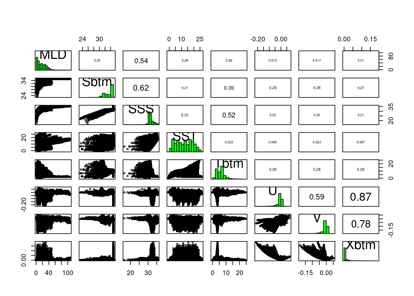
In the lower left portion of the plot we see paired scatter plots, at upper right we see the correlation values of the pairs, and long the diagonal we see a histogram of each variable. Some pairs are highly correlated, say over 0.7, and to include both in the modeling might not provide us with greater predictive power. It may feel counter intuitive to remove any variables - more data means more information, right? And more information means more informed models. Consider two measurements, human arm length and inseam. We might use these to predict if a person is tall, but since they are probably strongly collinear/correlated do we really need both?
2.3 Identify the most independent variables (and the most collinear)
We have a function that can help use select which variables to remove. filter_collinear() returns a listing of variables it suggests we keep. It attaches to the return value an attribute (like a post-it note stuck on a box) that lists the complementary variables that it suggests we drop. We are choosing a particular method, but you can learn more about using R’s help for ?filter_collinear.
keep = filter_collinear(present, method = "cor_caret", cutoff = 0.65)
keep
[1] "SSS" "U" "Sbtm" "V" "Tbtm" "MLD" "SST"
attr(,"to_remove")
[1] "Xbtm"drop_me = attr(keep, "to_remove")
drop_me[1] "Xbtm"Of course, we can decide to ignore this advice, and pick which ever ones we want including keeping them all. In fact, marine ecologists are loathe to drop depth; in coastal science in particular depth plays a significant role in ecology and biology. And we are modeling across the year, so we’ll include month as a variable that can be important.
keep = c("depth", "month", keep)Whatever selection of variables we decide to model with, we will save this listing to a file. That way we can refer to it programmatically, but that comes later.
2.4 A closer look at the model input data
Before we do commit to a selection of variables, let’s turn our attention back to our presence-background points, and look at just those chosen values rather than at values drawn form across the entire domain. Let’s open the file that contain our presence-background data during the PRESENT climate scenario.
model_input = read_model_input(scientificname = "Mola mola")
model_input
Simple feature collection with 14521 features and 2 fields
Geometry type: POINT
Dimension: XY
Bounding box: xmin: -74.72716 ymin: 38.84118 xmax: -65.00391 ymax: 45.1333
Geodetic CRS: WGS 84
# A tibble: 14,521 × 3
month class geom
<fct> <fct> <POINT [°]>
1 Jan presence (-71.989 39.668)
2 Jan presence (-69.62994 43.65584)
3 Jan presence (-67.79617 42.75941)
4 Jan presence (-71.31 41.49)
5 Jan presence (-72.05151 39.07928)
6 Jan background (-66.50078 42.33478)
7 Jan background (-72.5883 40.44271)
8 Jan background (-69.21549 41.5944)
9 Jan background (-72.91736 39.37328)
10 Jan background (-69.05096 39.7846)
# ℹ 14,511 more rowsAnd let’s read the covariate data again, but this time we’ll add depth. We won’t drop any variables, like Xbtm, just yet - we can do that later.
present = read_brickman(add = c("depth"))Next we’ll extract data values from our covariates.
variables = extract_brickman(present, model_input, form = "wide")
variables
Simple feature collection with 14521 features and 12 fields
Geometry type: POINT
Dimension: XY
Bounding box: xmin: -74.72716 ymin: 38.84118 xmax: -65.00391 ymax: 45.1333
Geodetic CRS: WGS 84
# A tibble: 14,521 × 13
.id month class depth MLD Sbtm SSS SST Tbtm U V
<chr> <fct> <fct> <dbl> <dbl> <dbl> <dbl> <dbl> <dbl> <dbl> <dbl>
1 p00001 Jan presence 231. 26.6 35.0 32.0 7.58 8.77 -3.48e-3 -4.36e-3
2 p00002 Jan presence 80.6 31.9 32.7 31.4 3.76 5.68 -6.15e-3 3.85e-5
3 p00003 Jan presence 192. 34.8 34.7 30.8 3.82 7.55 4.74e-3 1.64e-3
4 p00004 Jan presence 13.6 10.7 30.9 30.8 4.57 4.66 -8.93e-4 2.45e-2
5 p00005 Jan presence 2116. 45.9 35.0 33.3 10.9 3.72 7.56e-3 -6.58e-2
6 p00006 Jan backgrou… 269. 26.1 34.8 30.6 4.15 7.40 1.65e-2 5.86e-3
7 p00007 Jan backgrou… 45.4 40.8 31.9 31.7 6.35 6.83 6.76e-4 1.83e-3
8 p00008 Jan backgrou… 155. 44.3 34.1 31.2 4.46 7.12 9.94e-4 -2.15e-3
9 p00009 Jan backgrou… 70.1 34.0 33.6 31.9 7.44 10.4 -5.24e-3 -1.13e-2
10 p00010 Jan backgrou… 1947. 27.1 35.0 32.2 7.95 3.67 -1.42e-1 -4.53e-2
# ℹ 14,511 more rows
# ℹ 2 more variables: Xbtm <dbl>, geom <POINT [°]>We are going to call a plotting function, plot_pres_vs_bg(), that wants some of the data from model_input and some of the data in variables. So, we have to do some data wrangling to combine those; we’ll add class to variables and then drop the .id column.
variables = variables |>
  mutate(class = model_input$class) |>    # the $ extracts a column
  select(-.id)                            # the minus means "deselect" or "drop"
variables
Simple feature collection with 14521 features and 11 fields
Geometry type: POINT
Dimension: XY
Bounding box: xmin: -74.72716 ymin: 38.84118 xmax: -65.00391 ymax: 45.1333
Geodetic CRS: WGS 84
# A tibble: 14,521 × 12
month class depth MLD Sbtm SSS SST Tbtm U V Xbtm
<fct> <fct> <dbl> <dbl> <dbl> <dbl> <dbl> <dbl> <dbl> <dbl> <dbl>
1 Jan presence 231. 26.6 35.0 32.0 7.58 8.77 -3.48e-3 -4.36e-3 1.98e-3
2 Jan presence 80.6 31.9 32.7 31.4 3.76 5.68 -6.15e-3 3.85e-5 2.19e-3
3 Jan presence 192. 34.8 34.7 30.8 3.82 7.55 4.74e-3 1.64e-3 1.78e-3
4 Jan presence 13.6 10.7 30.9 30.8 4.57 4.66 -8.93e-4 2.45e-2 8.96e-3
5 Jan presence 2116. 45.9 35.0 33.3 10.9 3.72 7.56e-3 -6.58e-2 2.82e-2
6 Jan backgro… 269. 26.1 34.8 30.6 4.15 7.40 1.65e-2 5.86e-3 6.32e-3
7 Jan backgro… 45.4 40.8 31.9 31.7 6.35 6.83 6.76e-4 1.83e-3 6.92e-4
8 Jan backgro… 155. 44.3 34.1 31.2 4.46 7.12 9.94e-4 -2.15e-3 8.39e-4
9 Jan backgro… 70.1 34.0 33.6 31.9 7.44 10.4 -5.24e-3 -1.13e-2 4.45e-3
10 Jan backgro… 1947. 27.1 35.0 32.2 7.95 3.67 -1.42e-1 -4.53e-2 9.49e-2
# ℹ 14,511 more rows
# ℹ 1 more variable: geom <POINT [°]>Finally, can make a specialized plot comparing our variables for each class: presence and background. We’ll drop month temporarily since we can do a simply tally of those.
plot_pres_vs_bg(variables |> select(-month), "class")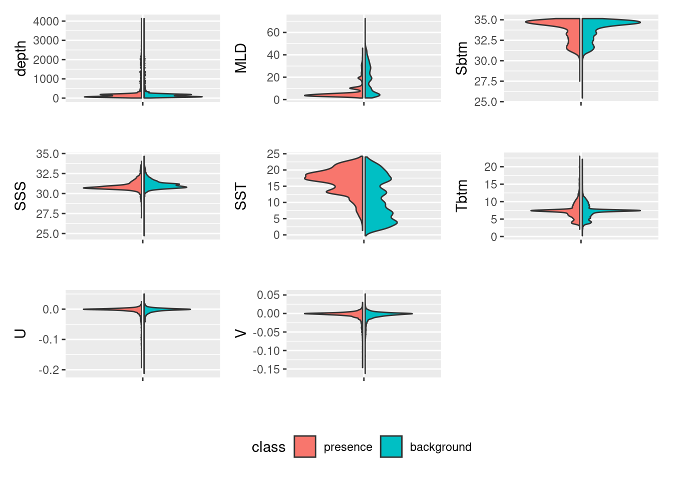
How does this inform our thinking about reducing the number of variables? For which variables do presence and background values mirror each other? Which have the least overlap? We know that the model works by finding optimal combinations of covariates for the species. If there is never a difference between the conditions for presences and background then how will it find the optimal niche conditions? Good questions!
2.5 Saving a file to keep track of modeling choices
You may have noticed that we write a lot of things to files (aka, “writing to disk”). It’s a useful practice especially when working with a multi-step process. One particular file, a configuration file, is used frequently in data science to store information about the choices we make as we work through our project. Configuration files generally are simple text files that we can easily get the computer to read and write.
In R, a confguration is treated as a named list. Each element of a list is named, but beyond that there aren’t any particular rules about configurations. You can learn more about configurations in this tutorial.
Let’s make a configuration list that holds 4 items: version identifier (“v1”), species name, the background selection scheme and the names of the variables to model with.
cfg = list(
  version = "v1",
  scientificname = "Mola mola",
  background = "average of observations per month",
  keep_vars =  keep)
We can access by name three ways using what is called “indexing” : using the [[ indexing brackets, using the $ indexing operator or using the getElement() function.
cfg[['scientificname']][1] "Mola mola"cfg[[2]][1] "Mola mola"cfg$scientificname[1] "Mola mola"getElement(cfg, "scientificname")[1] "Mola mola"getElement(cfg, 2)[1] "Mola mola"Now we’ll write this list to a file. First let’s set up a path where we might store these configurations, and for that matter, to store our modeling files. We’ll make a new directory, models/Aug and write the configuration there. We’ll use the famous “YAML” format to store the file. See the file functions/configuration.R for documentation on reading and writing.
ok = make_path(data_path("models")) # make a directory for models
write_configuration(cfg)
Let’s also save the now updated model_input data (it now includes covariate data for our version “v1”). Keep in mind that this contains all possible covariates (in out case that means we include Xbtm) even though we may drop one or more in subsequent steps.
write_model_input(variables, scientificname = "Mola mola", version = "v1")Use the Files pane to navigate to your personal data directory. Open the .yaml file - this is what your configuration looks like in YAML. Fortunately we don’t mess by hand with these much.
version: v1
scientificname: Mola mola
background: mean
keep_vars:
- depth
- month
- SSS
- U
- Sbtm
- V
- Tbtm
- MLD
- SST
3 Recap
We loaded the covariates for the “PRESENT” climate scenario and looked at collinearity across the entire study domain. We invoked a function that suggests which variables to keep and which to drop based upon collinearity. We examined the covariates at just the presence and background locations. We then saved a configuration for later reuse.
4 Coding Assignment C03
Select a second species to download and build both a configuration file and a model input file. Consider a species that is complimentary to your first species. For instance, in our example we selected a grazer of gelatinous creatures for our first species, so we might chose the second species to a type of gelatinous creature. But it should complimentary in other ways, too, such as temporal and spatial extent.
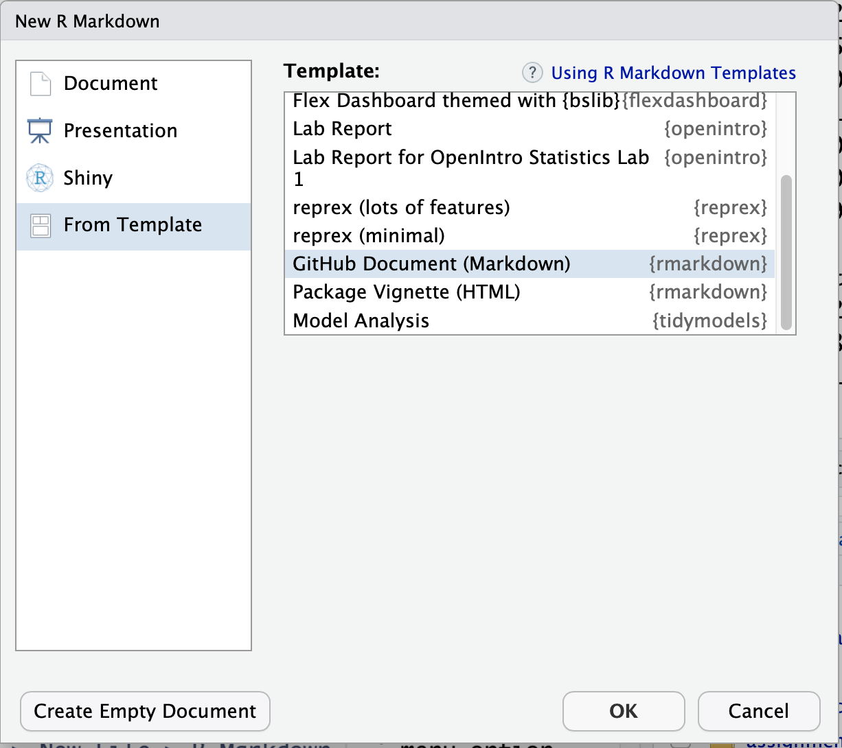
Record your steps in an R markdown file using the File > New File > R Markdown... menu option. Be sure to select the “GitHub Document (Markdown)” template. This will ensure that your work will render on your github page properly.
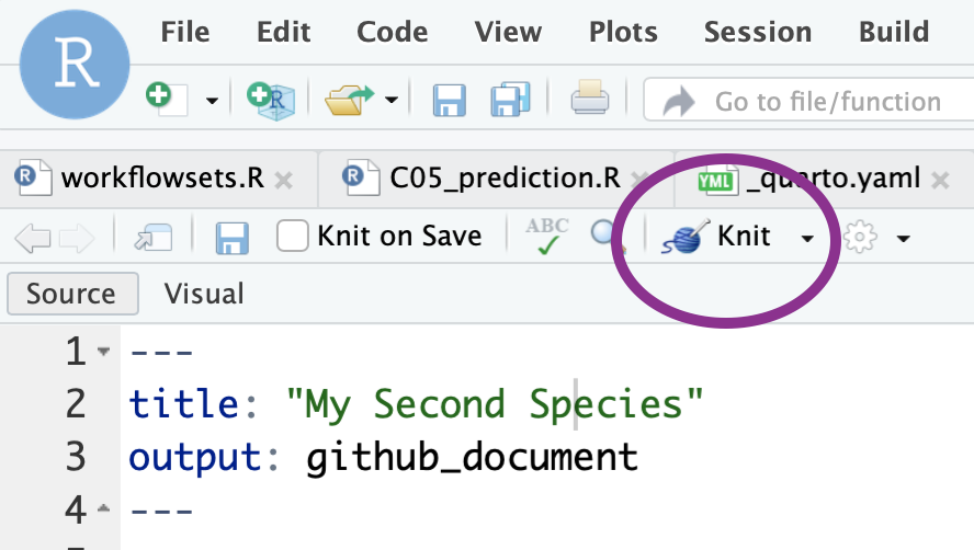
 Call the file ‘C03_assignment.Rmd’. Complete the steps necessary to download a species, create a configuration file and a model input file. Since you have a different species name but all of the parameters will be the same, you can continue to use ‘v1’ as the version identifier. At any time you can render the R Markdown to plain vanilla to a plain github-ready markdown text file by selecting the “knit” button.
 > Hint! R markdown files run the directory where they are stored. So, if you save ‘C03_assignment.Rmd’ at the top level of the directory you will be fine. If you save it somewhere else, like
 assignments, you will have to adjust the path to the setup file when you call source("setup.R") to something that provides the full path. Try this source("/home/<username>/<project_folder>/setup.R"), but, of course, user the proper username and project_folder values.
Another hint! You customized the function
read_observations()for your first species. Keep in mind you can always have species specific functions likeread_molamola()andread_humpback()if it makes life easier. Your call!
Lastly, commit your work and push the changes to your own github repository.