source("setup.R")Prediction
- It’s tough to make predictions, especially about the future.
- Yogi Berra
Finally we come to the end product of forecasting: prediction. This last step is actually fairly simple, given a recipe and model (now bundled in a workflow container). We want to predict across the entire domain of our Brickman data set. You may recall that we are able to read these arrays, display them and extract point data from them. But we haven’t used them en mass as a variable yet.
1 Setup
As always, we start by running our setup function. Start RStudio/R, and reload your project with the menu File > Recent Projects.
2 Load the Brickman data
We are going to make a prediction about the present, which means it something akin to a nowcast.
cfg = read_configuration(scientificname = "Mola mola",
                         version = "v1",
                         path = data_path("models"))
db = brickman_database()
db = brickman_database()
present_conditions = read_brickman(db |> filter(scenario == "PRESENT",
                                                interval == "mon"),
                       add = c("depth", "month")) |>
  select(all_of(cfg$keep_vars))
3 Load the workflow
We read the model information we created last time.
model_fits = read_model_fit(filename = "Mola_mola-v1-model_fits")
model_fits
# A tibble: 4 × 7
wflow_id splits id .metrics .notes .predictions .workflow
<chr> <list> <chr> <list> <list> <list> <list>
1 default_… <split [11230/3291]> trai… <tibble> <tibble> <tibble> <workflow>
2 default_… <split [11230/3291]> trai… <tibble> <tibble> <tibble> <workflow>
3 default_… <split [11230/3291]> trai… <tibble> <tibble> <tibble> <workflow>
4 default_… <split [11230/3291]> trai… <tibble> <tibble> <tibble> <workflow>4 Make a prediction
First we shall make a “nowcast” which is just a prediction of the current environmental conditions.
4.1 Nowcast
First make the prediction using predict_stars(). The function yields a stars array object that has one attribute (variable) for each row in the model_fits table. We simply provide the covariates (predictor variables) and the fu nction takes care of the rest.
nowcast = predict_stars(model_fits, present_conditions)
nowcast
stars object with 3 dimensions and 4 attributes
attribute(s):
Min. 1st Qu. Median Mean 3rd Qu.
default_glm 2.220446e-16 2.220446e-16 2.220446e-16 0.000471132 2.220446e-16
default_rf 1.389655e-03 1.012484e-01 2.678384e-01 0.305168340 4.768624e-01
default_btree 5.587810e-03 1.122404e-01 1.122404e-01 0.187268805 2.249077e-01
default_maxent 4.468855e-03 7.133545e-02 3.710900e-01 0.371976974 6.705825e-01
Max. NA's
default_glm 0.2751288 59796
default_rf 0.9150334 59796
default_btree 0.6669037 0
default_maxent 0.8744789 59796
dimension(s):
from to offset delta refsys point values x/y
x 1 121 -74.93 0.08226 WGS 84 FALSE NULL [x]
y 1 89 46.08 -0.08226 WGS 84 FALSE NULL [y]
month 1 12 NA NA NA NA Jan,...,Dec Now we can plot what is often called a “habitat suitability index” (hsi) map. We can
plot_prediction(nowcast['default_btree'])numeric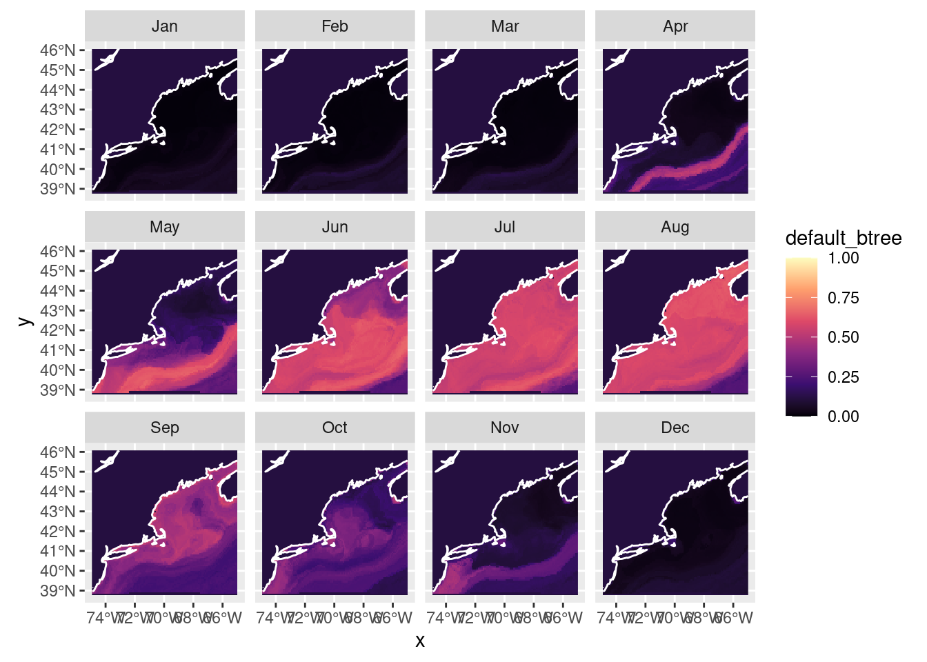
We can also plot a presence/absence labeled map, but keep in mind it is just a thresholded version of the above where “presence” means prediction >= 0.5. Of course, you can select other values to threshold the habitat suitablility scores.
pa_nowcast = threshold_prediction(nowcast)
plot_prediction(pa_nowcast['default_btree'])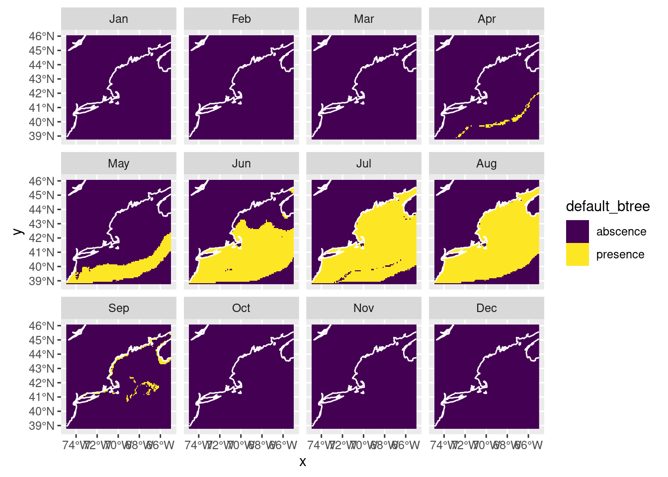
4.2 Forecast
Now let’s try our hand at forecasting - let’s try RCP85 in 2075. First we load those parameters, then run the prediction and plot.
covars_rcp85_2075 = read_brickman(db |> filter(scenario == "RCP85",
                                               year == 2075,
                                               interval == "mon"),
                                  add = c("depth", "month")) |>
  select(all_of(cfg$keep_vars))
forecast_2075 = predict_stars(model_fits, covars_rcp85_2075)
forecast_2075stars object with 3 dimensions and 4 attributes
attribute(s):
Min. 1st Qu. Median Mean
default_glm 2.220446e-16 2.220446e-16 2.220446e-16 0.0004014874
default_rf 5.175967e-03 1.416608e-01 3.154026e-01 0.3230973382
default_btree 6.479263e-03 1.122404e-01 1.122404e-01 0.1920485424
default_maxent 4.829635e-03 1.412765e-01 4.039507e-01 0.4038775395
3rd Qu. Max. NA's
default_glm 2.220446e-16 0.2376674 59796
default_rf 4.958535e-01 0.9061301 59796
default_btree 2.385872e-01 0.6728659 0
default_maxent 6.705062e-01 0.8916939 59796
dimension(s):
from to offset delta refsys point values x/y
x 1 121 -74.93 0.08226 WGS 84 FALSE NULL [x]
y 1 89 46.08 -0.08226 WGS 84 FALSE NULL [y]
month 1 12 NA NA NA NA Jan,...,Dec plot_prediction(forecast_2075['default_btree'])numeric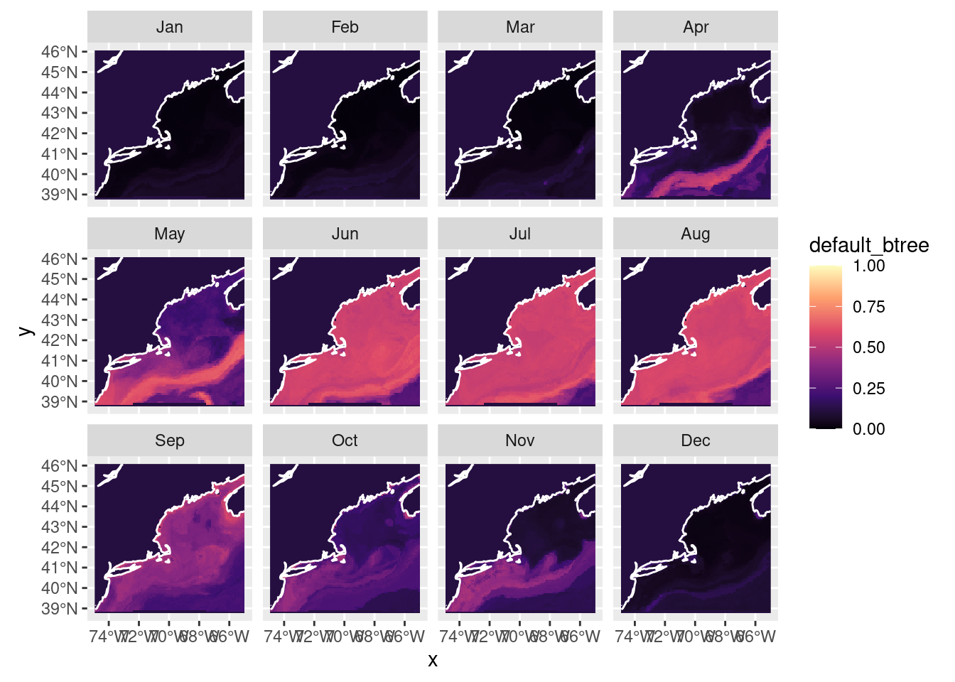
Note
Don’t forget that there are other ways to plot array based spatial data.
4.3 Save the predictions
It’s easy to save the predictions (and read then back with read_prediction()).
# make sure the output directory exists
path = make_path("predictions")

write_prediction(nowcast,
                 scientificname = cfg$scientificname,
                 version = cfg$version,
                 year = "CURRENT",
                 scenario = "CURRENT")
write_prediction(forecast_2075,
                 scientificname = cfg$scientificname,
                 version = cfg$version,
                 year = "2075",
                 scenario = "RCP85")
5 Recap
We made both a nowcast and a predictions using previously saved model fits. Contrary to Yogi Berra’s claim, it’s actually pretty easy to predict the future. Perhaps more challenging is to interpret the prediction. We bundled these together to make time series plots, and we saved the predicted values.
6 Coding Assignment
For each each climate scenario create a monthly forecast (so that’s three time periods: PRESENT, 2055 and 2075 and three scenarios CURRENT, RCP45, RCP85) and save each to in your predictions directory. In the end you should have 5 files saved (one for PRESENT and two each for 2055 and 2075).
Do the same for your second species. Ohhh, perhaps this a good time for another R markdown or R script to keep it all straight?