source("setup.R", echo = FALSE)
suppressPackageStartupMessages(library(tidysdm))
bb = get_bb(form = 'polygon')
coast = rnaturalearth::ne_coastline(scale = 'large', returnclass = 'sf') |>
  sf::st_geometry()
obs = read_obis() |>
dplyr::filter(date >= as.Date("2000-01-01"))Data thinning
1 Thinning the observations
Here we thin the data. The idea of thinning is to have one presence point per cell of the target raster output. For this purpose we’ll need not just the observation data, but also a raster of the desired extent and resolution. We have two rasterized covariate datasets we can load in, and then use one or the other as our template.
First, the observations…
And now the covariates…
sst_path = "data/oisst"
sst_db = oisster::read_database(sst_path) |>
  dplyr::arrange(date)

wind_path = "data/nbs"
wind_db = nbs::read_database(wind_path) |>
  dplyr::arrange(date)

preds = read_predictors(sst_db = sst_db,
                        windspeed_db = wind_db |> dplyr::filter(param == "windspeed"),
                        u_wind_db = wind_db |> dplyr::filter(param == "u_wind"),
v_wind_db = wind_db |> dplyr::filter(param == "v_wind"))We actually provide a simpler method for loading the the predictor variables as raster. In the future you may see this preds = read_predictors(quick = TRUE).
We’ll take the first slice of sst as a template and convert it into a mask. We’ll also save the mask for later use.
mask = dplyr::slice(preds['sst'], "time", 1) |>
  rlang::set_names("mask")|>
  dplyr::mutate(mask = factor(c("mask", NA_character_)[as.numeric(is.na(mask) + 1)],
                              levels = "mask")) |>
  stars::write_stars("data/mask/mask_factor.tif")

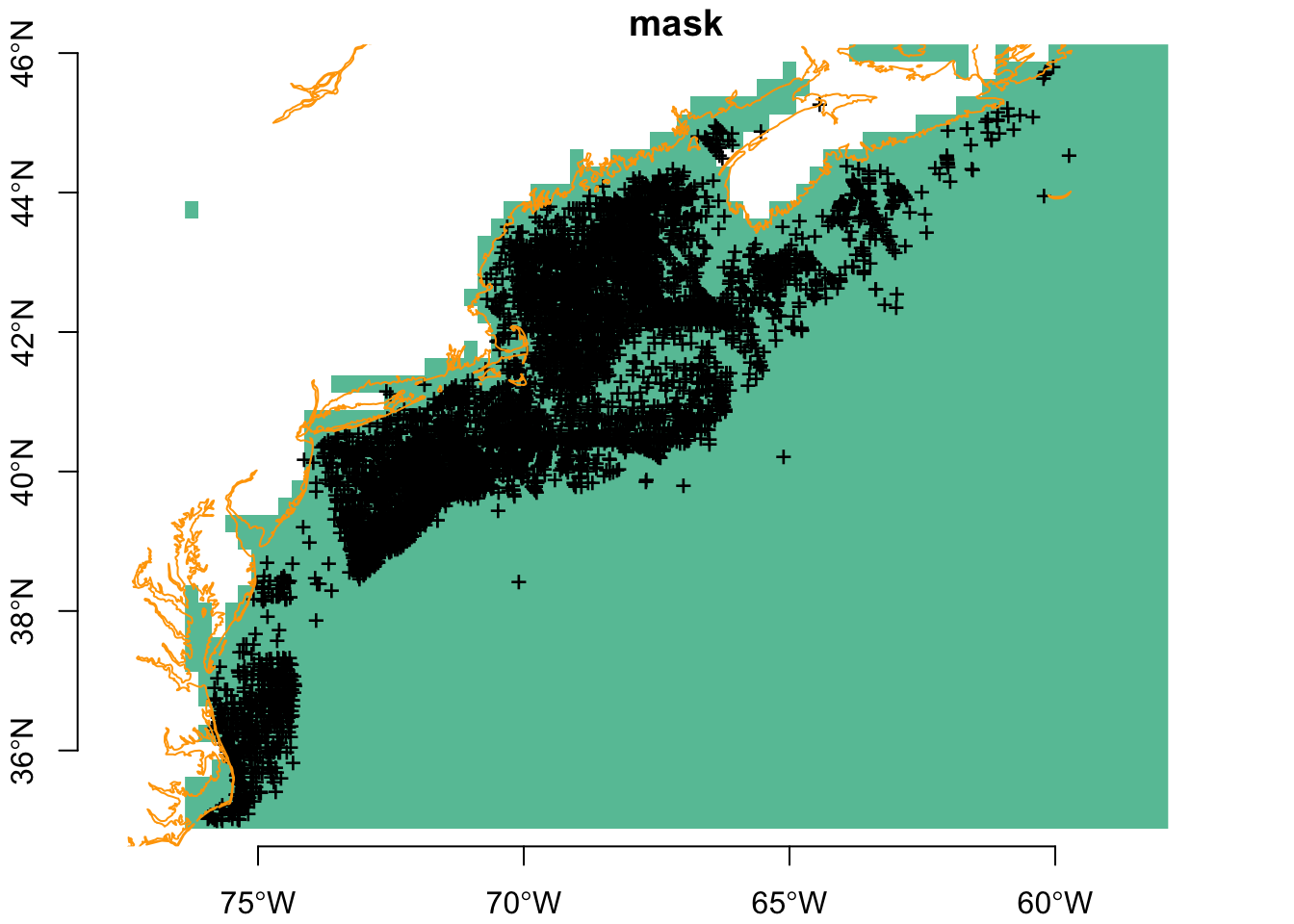
plot(mask, breaks = "equal", axes = TRUE, reset = FALSE)
plot(sf::st_geometry(obs), pch = "+", add = TRUE)
plot(coast, col = "orange", add = TRUE)
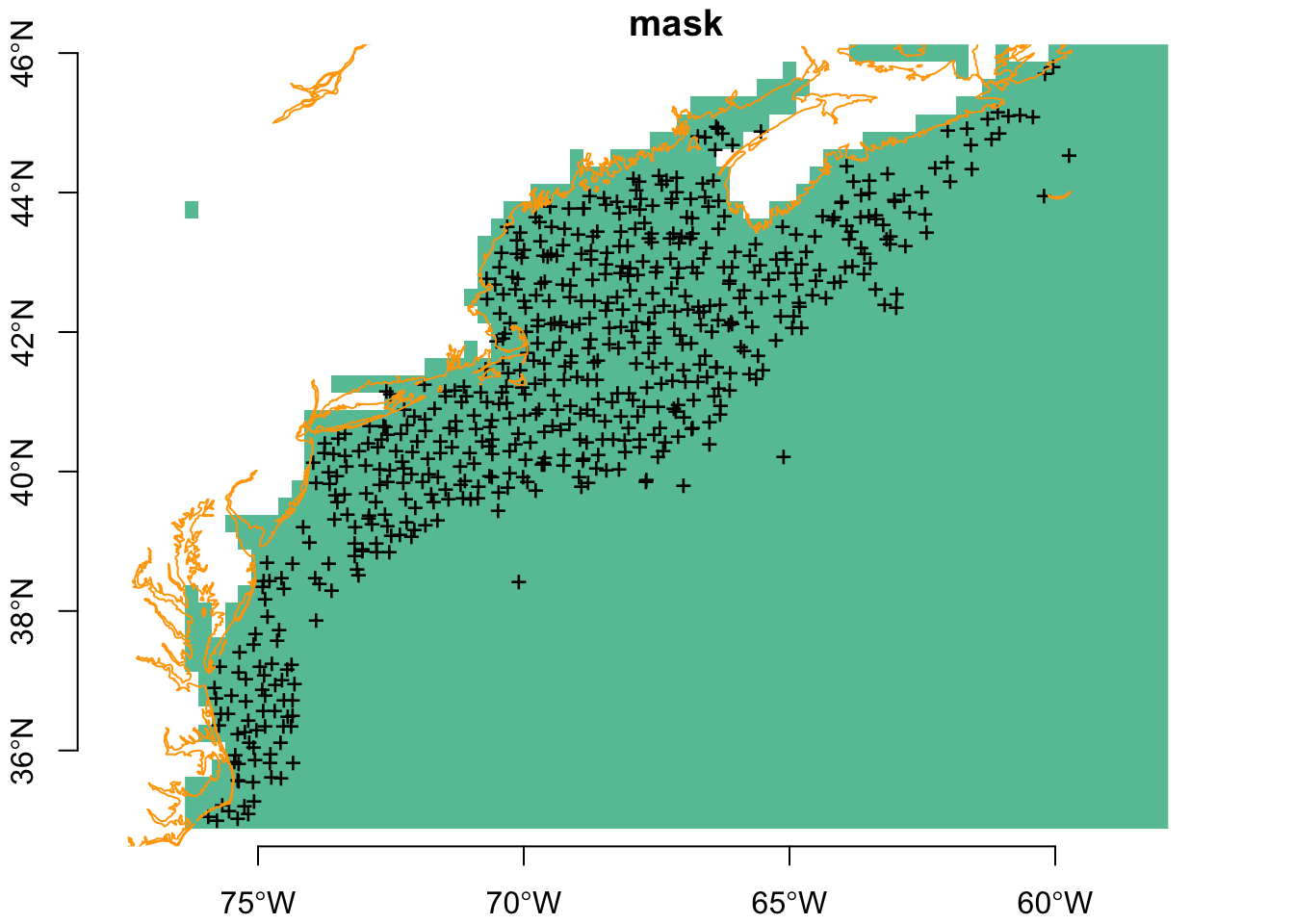
Now we can thin using thin_by_cell(). You can see the number of observations is greatly winnowed.
set.seed(1234)
thinned_obs <- tidysdm::thin_by_cell(obs, raster = mask)
plot(mask, breaks = "equal", axes = TRUE, reset = FALSE)
plot(sf::st_geometry(thinned_obs), pch = "+", add = TRUE)
plot(coast, col = "orange", add = TRUE)
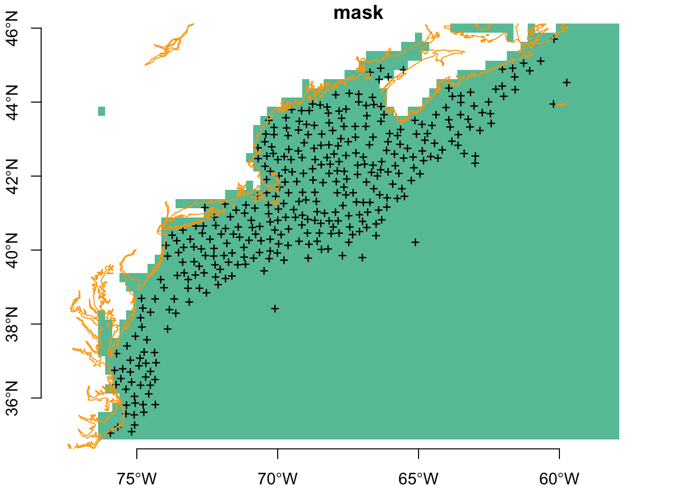
Next is to thin again by separation distance. Note that now thins even more more observation points. We’ll also save these for later reuse.
thinned_obs <- tidysdm::thin_by_dist(thinned_obs, dist_min = km2m(20)) |>
  sf::write_sf("data/obs/thinned_obs.gpkg")
plot(mask, breaks = "equal", axes = TRUE, reset = FALSE)
plot(sf::st_geometry(thinned_obs), pch = "+", add = TRUE)
plot(coast, col = "orange", add = TRUE)