source("setup.R")
bb = get_bb(form = 'polygon')
coast = rnaturalearth::ne_coastline(scale = 'large', returnclass = 'sf') |>
  sf::st_geometry()
thinned_obs = read_obs("thinned_obs")
obs = read_obs("obis")
mask = read_mask()
preds = read_predictors(quick = TRUE)Background sampling
1 Sampling background
Here we depart a little from the original workflow to use the full compliment of observations to generate a sampling bias map. We diverge from the original workflow because we have no observations of “similar species” - Mola mola is unique.
Note that we read in a number objects that we saved earlier. We only to this to manage the rendering of the webpage.
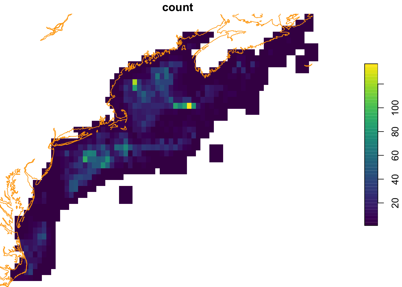
First we develop a sampling density map to guide the backgroud selection if there is a sampling bias. We provide a function that takes a set of spatial points and a raster defining the desired geometry, and returns a raster with the number of points per cell.
We expand the sample region by dilating the region (padding with 1) using a binary image processing step. This is not usually required, and may not be justified, but for the purpose of this tutorial it allows us to develop a reasonable selection of background points.
observation_density_raster = rasterize_point_density(obs, mask, dilate = 3)
pal = terra::map.pal("viridis", 50)
plot(observation_density_raster,
     col = pal,
     nbreaks = length(pal) + 1,
     breaks = "equal",
     reset = FALSE)
plot(coast, col = "orange", add = TRUE) 
Ahhh, as you might have surmised, there are some places where observations occur more frequently than in other places (observer bias? or species niche selection?) Now we select random background points using this weighted map to guide the background point selection.
And we could dive into the endlessly fun discussion about what are we trying to do here? We know that selecting points at random is aimed at providing the model information that characterizes the backgound. After all, ultimately the model is used discriminate likely habitat relative to unlikely habitat. But… are we characterizing background just near the where observations occur? Or are we characterizing the background across the entire domain of the study? An endlessly fun topic for dinner parties!
set.seed(1234)
model_input <- tidysdm::sample_background(
    data = thinned_obs,
    raster = observation_density_raster,
    n = 2*nrow(thinned_obs),
    method = "bias",
    class_label = "background",
    return_pres = TRUE) |>
  dplyr::mutate(time = lubridate::NA_Date_, .after = 1)
ix <- model_input$class == "presence"
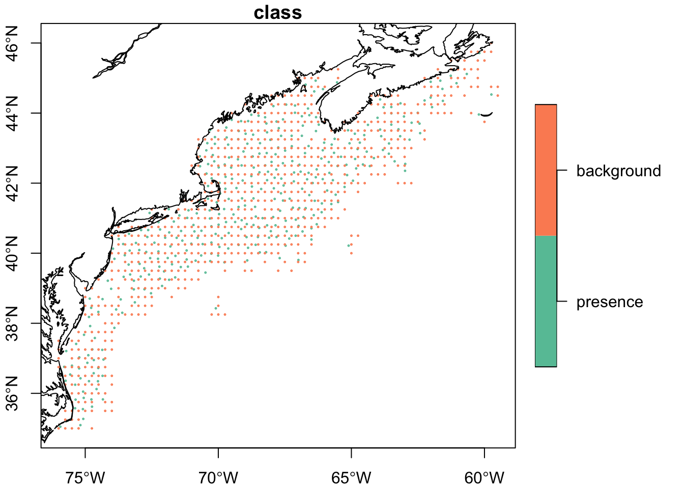
model_input$time[ix] <- oisster::current_month(thinned_obs$date)plot(model_input['class'], pch = 1, cex = 0.2,reset = FALSE, axes = TRUE)
plot(coast, col = "black", add = TRUE)
This is a different approach than we were not bound to the raster-covariates to select random background points - in fact we saturated the region of interest. It is worth considering the advantages and disadvantages of each - even before considering the statistical implications.
1.1 Sampling background time
Next we need to think about sampling through time for the background points. We’ll borrow from earlier work to make a weighted time sample.
set.seed(1234)
nback = sum(!ix)
days_sample = sample_time(obs$date,
                          size = nback,
                          by = "month",
                          replace = TRUE,
                          weighted = TRUE)
# recall ix is the logical identifying the class "presence"
model_input$time[!ix] <- days_sample
2 Extract points data from covariates
It’s easy to extract point data from raster. These we shall save for later use.
input_data = stars::st_extract(preds, at = model_input, time_column = "time") |>
  sf::st_as_sf() |>
  dplyr::as_tibble() |>
  dplyr::select(dplyr::all_of(names(preds)))
model_input = dplyr::bind_cols(model_input, input_data) |>
  dplyr::select(-dplyr::all_of("time")) |>
  dplyr::relocate(dplyr::all_of("class"), .before = 1) |>
  dplyr::glimpse()
Rows: 1,089
Columns: 6
$ class <fct> presence, presence, presence, presence, presence, presence, …
$ geometry <POINT [°]> POINT (-66.60798 42.2943), POINT (-68.00023 42.60569),…
$ sst <dbl> 12.45633, 20.16968, 14.89867, 18.12452, 16.69533, 27.77900, …
$ windspeed <dbl> 4.911994, 4.860674, 8.411347, 4.308283, 8.377000, 7.495667, …
$ u_wind <dbl> -0.27018008, 1.58849359, 2.05362248, 1.27765775, 0.86364067,…
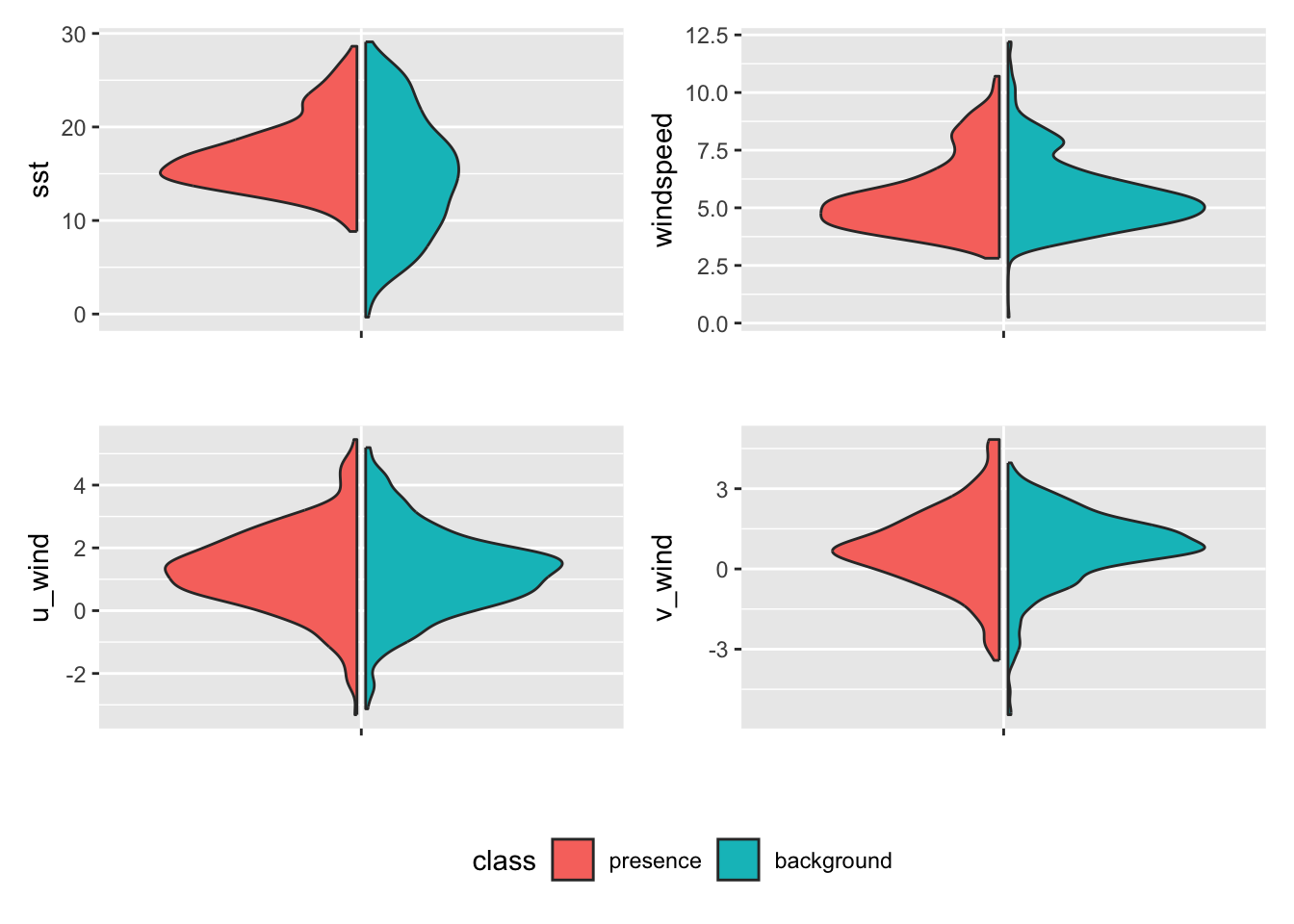
$ v_wind <dbl> -0.54305273, 0.75563574, -0.73934704, 2.79159832, -1.1114074…Now let’s look at the relationships among these predicitors. These comparisons seem valuable, but requires some study to understand their importance. First a distribution plot. Here the data are divided into presence and background and side-by-side comparisons of the distributions are made.
model_input |>
  dplyr::select(dplyr::all_of(c("class", names(preds)))) |>
  tidysdm::plot_pres_vs_bg(class)
We can then compute a distance metric that measures the “distance” between presence and background records for a given covariate. The bigger the distance the more suitable the covariate is for modeling because a high distance tells us that the species occupies a distinctive niche within the available setting. Just what consitutes enough distance is harder to know. Clearly u_wind and windspeed variables will be weaker when it comes to discriminating suitable habitats compared to sst and v_wind.
model_input |>
  dplyr::select(dplyr::all_of(c("class", names(preds)))) |>
  tidysdm::dist_pres_vs_bg(class)
sst v_wind windspeed u_wind
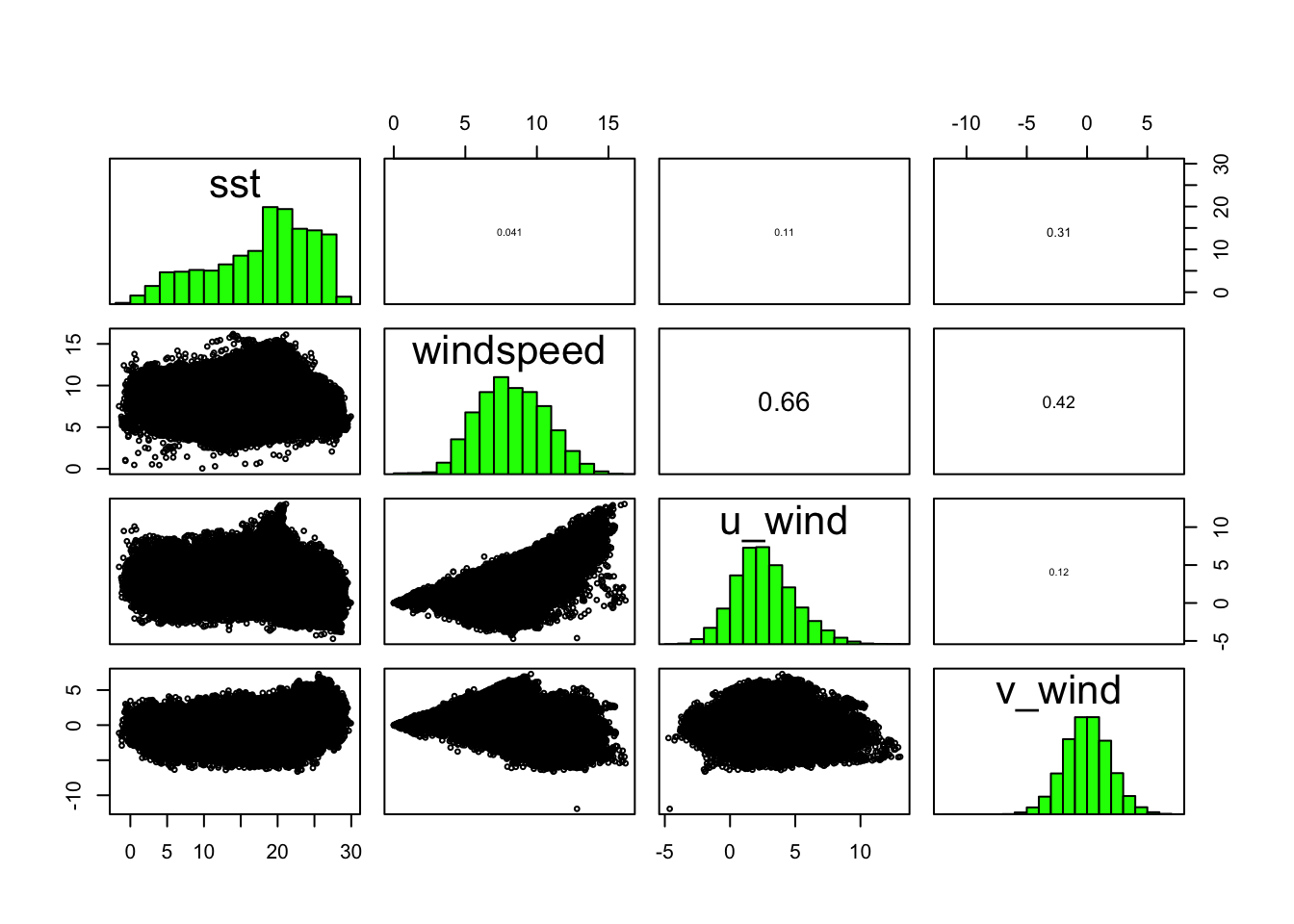
0.31422174 0.11752016 0.08002330 0.05547888 We can also look into correlations between the covariates. We might expect that windspeed, which is a function of u_wind and v_wind might correlatre with those. But what we find is that except for windspeed and u_wind (the east-west component of wind) there isn’t any obvious correlation.
pairs(preds)
We can also deploy a filtering function that will identify the uncorrelated covariates (and the correlated ones, too!) Noe that none are recommened for removal, so we proceed with all four. If any had been flagged for removal we would do just that.
vars_uncor <- tidysdm::filter_collinear(preds, cutoff = 0.7, method = "cor_caret", verbose = TRUE)All correlations <=0.7vars_uncor[1] "windspeed" "u_wind" "v_wind" "sst"
attr(,"to_remove")
character(0)OK - we’ll save these for later use.
model_input = dplyr::select(model_input,
                           dplyr::all_of(c("class", names(preds)))) |>
  sf::write_sf("data/obs/model_input.gpkg")