library(psptools)
library(pspdata)

library(dplyr)
library(ggplot2)
Class Imbalance
Class imbalance in training data using binary and multiclass bins
psp <- read_psp_data(model_ready=TRUE) Binary
Predicting probability of toxicity above/below closure limit
cfg <- list(
  configuration="test",
  image_list = list(tox_levels = c(0,80),
                    forecast_steps = 1,
                    n_steps = 2,
                    minimum_gap = 4,
                    maximum_gap = 10,
                    multisample_weeks="last",
                    toxins = c("gtx4", "gtx1", "dcgtx3", "gtx5", "dcgtx2", "gtx3",
                               "gtx2", "neo", "dcstx", "stx", "c1", "c2")),
  model = list(balance_val_set=FALSE,
               downsample=FALSE,
               use_class_weights=FALSE,
               dropout1 = 0.3,
               dropout2 = 0.3,
               batch_size = 32,
               units1 = 32,
               units2 = 32,
               epochs = 128,
               validation_split = 0.2,
               shuffle = TRUE,
               num_classes = 4,
               optimizer="adam",
               loss_function="categorical_crossentropy",
               model_metrics=c("categorical_accuracy")),
  train_test = list(split_by="year_region_species",
                    train = list(
                      year = c("2014", "2015", "2016", "2017", "2018", "2019", "2020", "2021", "2022", "2023", "2024"),
                      region = c("maine"),
                      species = c("mytilus")),
                    test = list(
                      year = c("2014"),
                      region= c("maine"),
                      species = c("mya")))
)
binary <- transform_data(cfg, psp)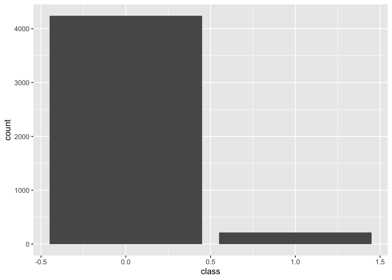
Multiclass
Predicting one of more than two toxicity classifications. Here we use 0, 10, 30, and 80 as cutoffs.
cfg <- list(
  configuration="test",
  image_list = list(tox_levels = c(0,10,30,80),
                    forecast_steps = 1,
                    n_steps = 2,
                    minimum_gap = 4,
                    maximum_gap = 10,
                    multisample_weeks="last",
                    toxins = c("gtx4", "gtx1", "dcgtx3", "gtx5", "dcgtx2", "gtx3",
                               "gtx2", "neo", "dcstx", "stx", "c1", "c2")),
  model = list(balance_val_set=FALSE,
               downsample=FALSE,
               use_class_weights=FALSE,
               dropout1 = 0.3,
               dropout2 = 0.3,
               batch_size = 32,
               units1 = 32,
               units2 = 32,
               epochs = 128,
               validation_split = 0.2,
               shuffle = TRUE,
               num_classes = 4,
               optimizer="adam",
               loss_function="categorical_crossentropy",
               model_metrics=c("categorical_accuracy")),
  train_test = list(split_by="year_region_species",
                    train = list(
                      year = c("2014", "2015", "2016", "2017", "2018", "2019", "2020", "2021", "2022", "2023", "2024"),
                      region = c("maine"),
                      species = c("mytilus")),
                    test = list(
                      year = c("2014"),
                      region= c("maine"),
                      species = c("mya")))
)
multiclass <- transform_data(cfg, psp)
Classification counts in training data through end of 2024
# A tibble: 4 × 3
  class     n proportion
  <dbl> <int>      <dbl>
1     0  6775      0.782
2     1   972      0.112
3     2   511      0.059
4     3   410      0.047
Techniques for overcoming class imbalance
Downsampling
The distribution of the classes becomes even. Since we only have around 200 samples in class 3 (the most rare), we will sample that many from each of the others.
cfg <- list(
  configuration="test",
  image_list = list(tox_levels = c(0,10,30,80),
                    forecast_steps = 1,
                    n_steps = 3,
                    minimum_gap = 4,
                    maximum_gap = 10,
                    multisample_weeks="last",
                    toxins = c("gtx4", "gtx1", "dcgtx3", "gtx5", "dcgtx2", "gtx3",
                               "gtx2", "neo", "dcstx", "stx", "c1", "c2")),
  model = list(balance_val_set=FALSE,
               downsample=TRUE,
               use_class_weights=FALSE,
               dropout1 = 0.3,
               dropout2 = 0.3,
               batch_size = 32,
               units1 = 32,
               units2 = 32,
               epochs = 128,
               validation_split = 0.2,
               shuffle = TRUE,
               num_classes = 4,
               optimizer="adam",
               loss_function="categorical_crossentropy",
               model_metrics=c("categorical_accuracy")),
  train_test = list(split_by="year_region_species",
                    train = list(
                      year = c("2015", "2016", "2017", "2018", "2019", "2020", "2021"),
                      region = c("maine"),
                      species = c("mytilus")),
                    test = list(
                      year = c("2014"),
                      region= c("maine"),
                      species = c("mytilus")))
)
downsampled <- transform_data(cfg, psp)tibble(location = downsampled$train$locations, class = downsampled$train$classifications) |>
ggplot(aes(x=class)) +
geom_bar()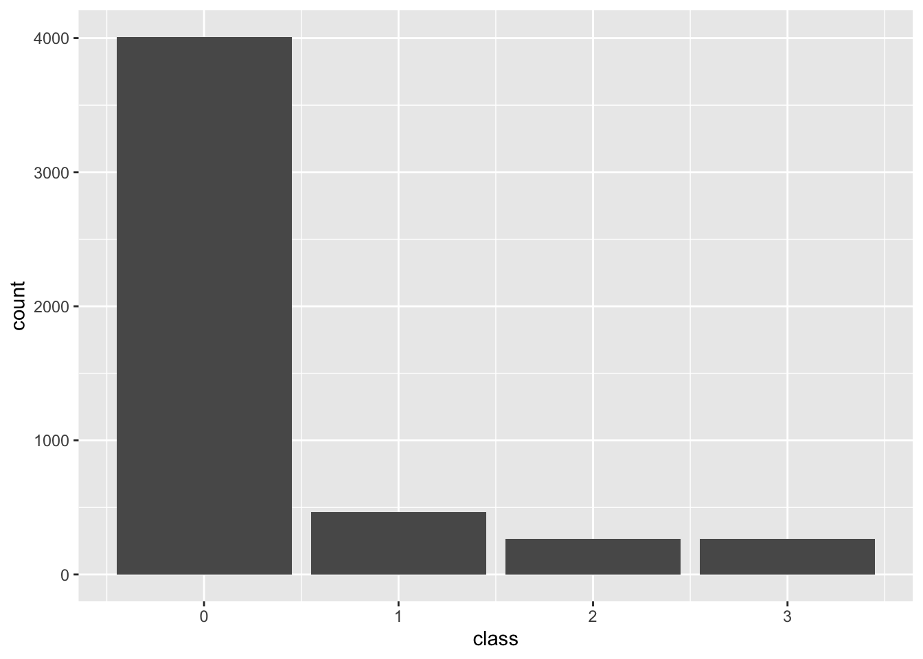
Validation set balancing
The keras::fit() function will let us manually assign the samples in the validation set, rather than choosing a random percentage with the validation_split argument. We can sample an even distribution of each class. Balancing the validation set can be combined with downsampling in the training set.
cfg <- list(
  configuration="test",
  image_list = list(tox_levels = c(0,10,30,80),
                    forecast_steps = 1,
                    n_steps = 3,
                    minimum_gap = 4,
                    maximum_gap = 10,
                    multisample_weeks="last",
                    toxins = c("gtx4", "gtx1", "dcgtx3", "gtx5", "dcgtx2", "gtx3",
                               "gtx2", "neo", "dcstx", "stx", "c1", "c2")),
  model = list(balance_val_set=TRUE,
               downsample=FALSE,
               use_class_weights=FALSE,
               dropout1 = 0.3,
               dropout2 = 0.3,
               batch_size = 32,
               units1 = 32,
               units2 = 32,
               epochs = 128,
               validation_split = 0.2,
               shuffle = TRUE,
               num_classes = 4,
               optimizer="adam",
               loss_function="categorical_crossentropy",
               model_metrics=c("categorical_accuracy")),
  train_test = list(split_by="year",
                    train = c("2015", "2016", "2017", "2018", "2019", "2020", "2021"),
                    test = c("2014"))
)
#balanced_val <- transform_data(cfg, psp)#str(balanced_val)#tibble(location = balanced_val$val$locations, class = balanced_val$val$classifications) |>
# ggplot(aes(x=class)) +
# geom_bar()Weighted classes
keras::fit() also accepts a class_weights argument. psptools provides a function get_class_weights() to obtain these.
cfg <- list(
  configuration="test",
  image_list = list(tox_levels = c(0,10,30,80),
                    forecast_steps = 1,
                    n_steps = 3,
                    minimum_gap = 4,
                    maximum_gap = 10,
                    multisample_weeks="last",
                    toxins = c("gtx4", "gtx1", "dcgtx3", "gtx5", "dcgtx2", "gtx3",
                               "gtx2", "neo", "dcstx", "stx", "c1", "c2")),
  model = list(balance_val_set=FALSE,
               downsample=FALSE,
               use_class_weights=TRUE,
               dropout1 = 0.3,
               dropout2 = 0.3,
               batch_size = 32,
               units1 = 32,
               units2 = 32,
               epochs = 128,
               validation_split = 0.2,
               shuffle = TRUE,
               num_classes = 4,
               optimizer="adam",
               loss_function="categorical_crossentropy",
               model_metrics=c("categorical_accuracy")),
  train_test = list(split_by="year_region_species",
                    train = list(
                      year = c("2015", "2016", "2017", "2018", "2019", "2020", "2021"),
                      region = c("maine"),
                      species = c("mytilus")),
                    test = list(
                      year = c("2014"),
                      region= c("maine"),
                      species = c("mytilus")))
)
model_input <- transform_data(cfg, psp)class_weights <- get_class_weights(model_input$train$classifications)
class_weights$`0`
[1] 1
$`1`
[1] 8.603004
$`2`
[1] 15.01498
$`3`
[1] 15.18561