Exploring the Input Data

glimpse(psp)

Rows: 14,800
Columns: 19
$ id             <chr> "PSP19.3_2014-04-01_mytilus", "PSP21.09_2014-04-01_myti…
$ location_id    <chr> "PSP19.3", "PSP21.09", "PSP21.2", "PSP25.17", "PSP26.07…
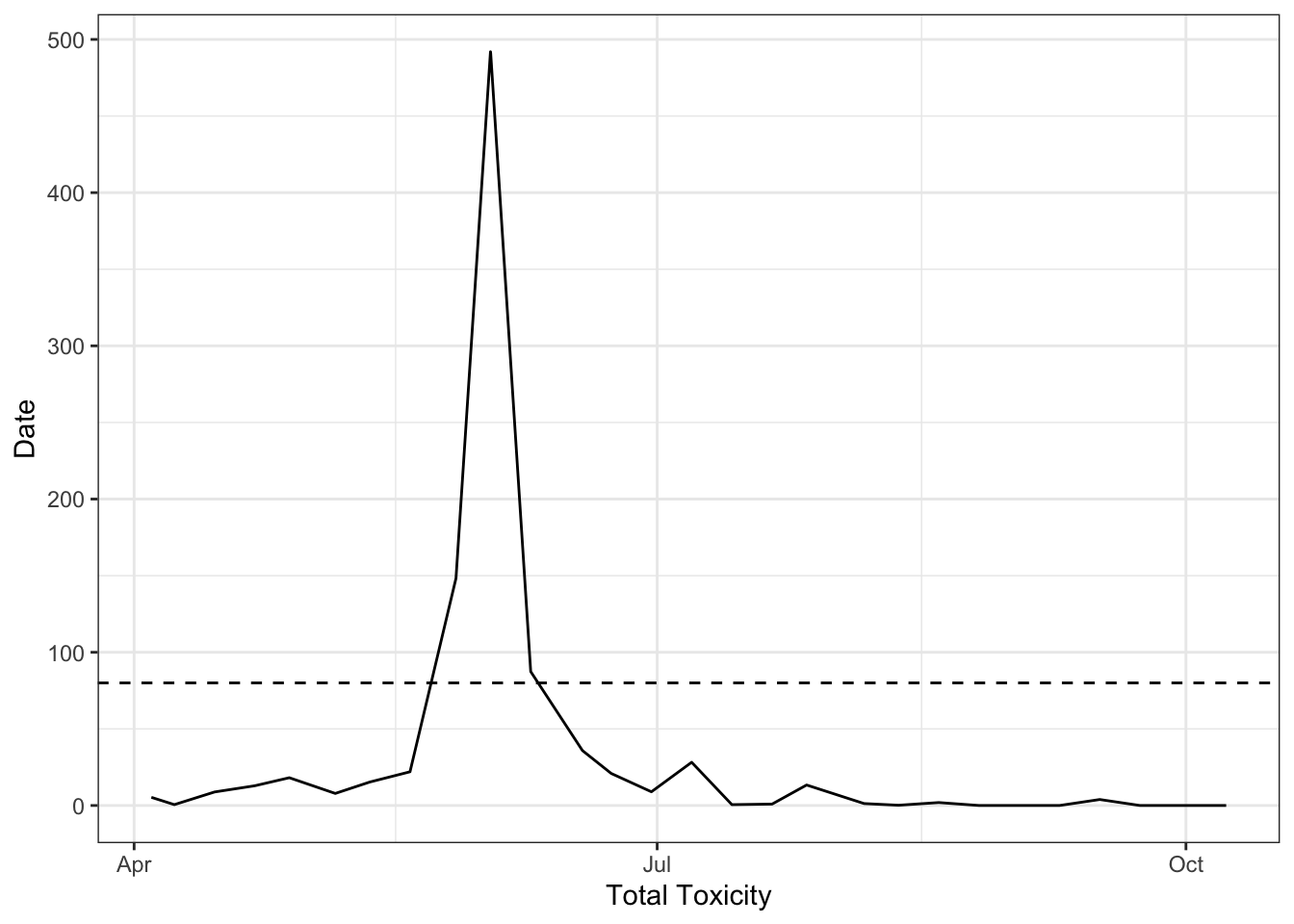
$ date           <date> 2014-04-01, 2014-04-01, 2014-04-01, 2014-04-02, 2014-0…
$ species        <chr> "mytilus", "mytilus", "mytilus", "mytilus", "mytilus", …
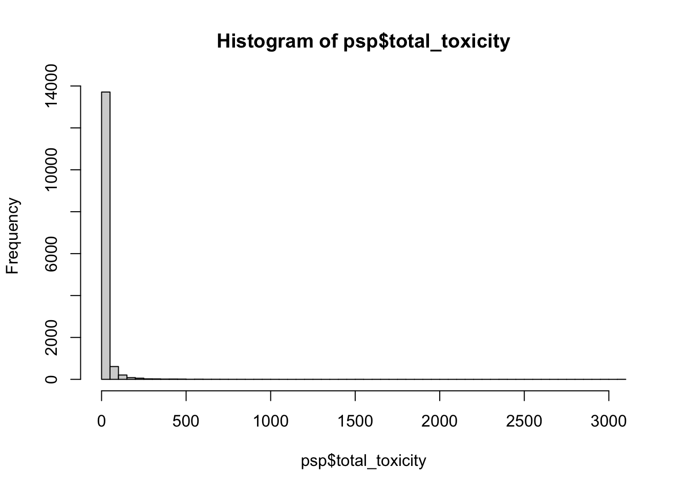
$ total_toxicity <dbl> 0.1561590, 0.2044939, 0.1933397, 0.1301325, 0.1859036, …
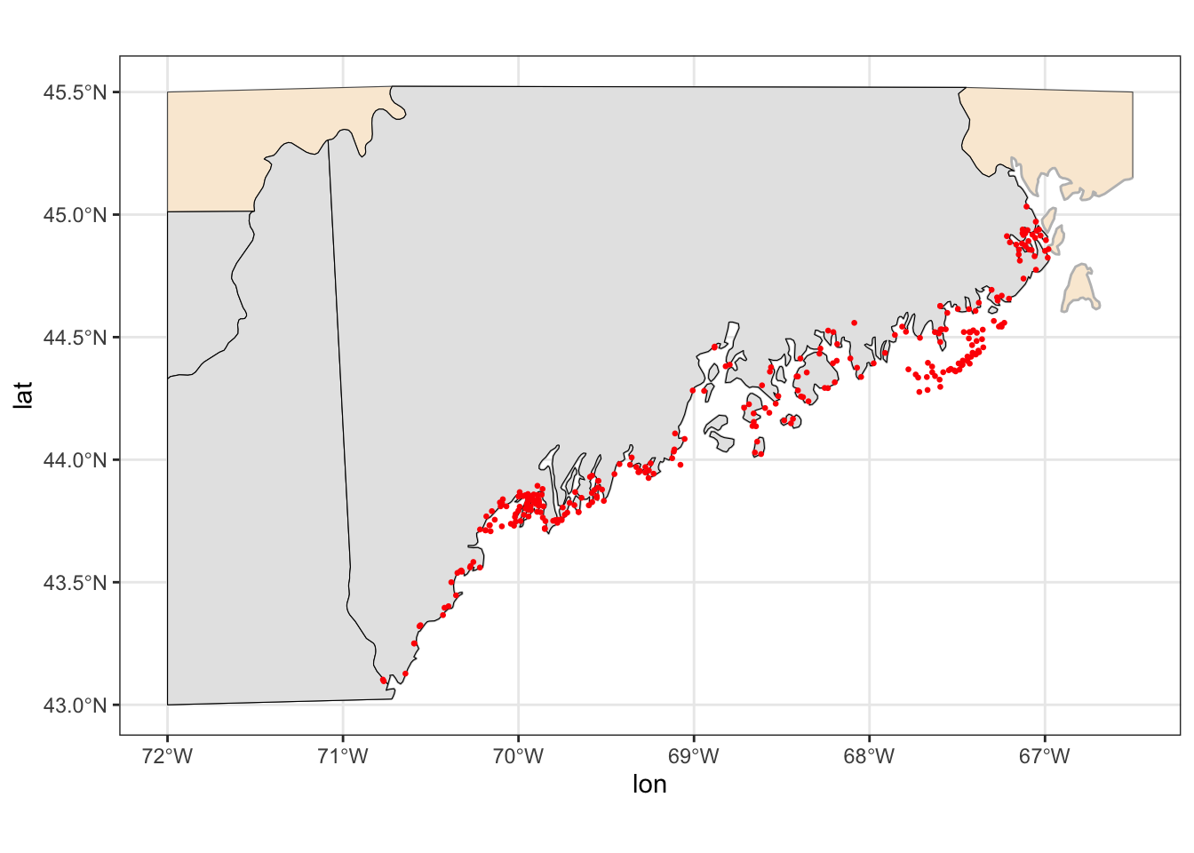
$ lat            <dbl> 44.22853, 44.23824, 44.29200, 44.61438, 44.65701, 44.53…
$ lon            <dbl> -68.53441, -68.34792, -68.23696, -67.43323, -67.20525, …
$ gtx4           <dbl> 0, 0, 0, 0, 0, 0, 0, 0, 0, 0, 0, 0, 0, 0, 0, 0, 0, 0, 0…
$ gtx1           <dbl> 0.000000, 0.000000, 0.000000, 0.000000, 0.000000, 0.000…
$ dcgtx3         <dbl> 0, 0, 0, 0, 0, 0, 0, 0, 0, 0, 0, 0, 0, 0, 0, 0, 0, 0, 0…
$ gtx5           <dbl> 0, 0, 0, 0, 0, 0, 0, 0, 0, 0, 0, 0, 0, 0, 0, 0, 0, 0, 0…
$ dcgtx2         <dbl> 0, 0, 0, 0, 0, 0, 0, 0, 0, 0, 0, 0, 0, 0, 0, 0, 0, 0, 0…
$ gtx3           <dbl> 0.1561590, 0.2044939, 0.1933397, 0.1301325, 0.1859036, …
$ gtx2           <dbl> 0, 0, 0, 0, 0, 0, 0, 0, 0, 0, 0, 0, 0, 0, 0, 0, 0, 0, 0…
$ neo            <dbl> 0, 0, 0, 0, 0, 0, 0, 0, 0, 0, 0, 0, 0, 0, 0, 0, 0, 0, 0…
$ dcstx          <dbl> 0, 0, 0, 0, 0, 0, 0, 0, 0, 0, 0, 0, 0, 0, 0, 0, 0, 0, 0…
$ stx            <dbl> 0.000000, 0.000000, 0.000000, 0.000000, 0.000000, 0.000…
$ c1             <dbl> 0, 0, 0, 0, 0, 0, 0, 0, 0, 0, 0, 0, 0, 0, 0, 0, 0, 0, 0…
$ c2             <dbl> 0, 0, 0, 0, 0, 0, 0, 0, 0, 0, 0, 0, 0, 0, 0, 0, 0, 0, 0…

The data set contains seasonal biotoxin measurements from 2014 until present

summary(psp$date)

        Min.      1st Qu.       Median         Mean      3rd Qu.         Max. 
"2014-04-01" "2015-07-15" "2017-07-09" "2018-03-12" "2020-05-18" "2024-09-11" 

There are >250 unique sampling locations along the Maine coast. Sites have been sampled between 1 and almost 300 times.

counts <- count(psp, location_id) |>
  arrange(desc(n))

counts

# A tibble: 383 × 2
   location_id     n
   <chr>       <int>
 1 PSP27.46      322
 2 PSP26.15      261
 3 PSP12.03      258
 4 PSP12.13      257
 5 PSP10.11      250
 6 PSP10.33      240
 7 PSP16.41      237
 8 PSP12.34      234
 9 PSP27.05      233
10 PSP12.01      228
# ℹ 373 more rows

hist(counts$n)

A map of all of the stations included in this tutorial

summary(psp$total_toxicity)

    Min.  1st Qu.   Median     Mean  3rd Qu.     Max. 
   0.000    0.000    1.121   16.531    8.935 3092.832 

hist(psp$total_toxicity, 100)

There are multiple shellfish species that are sampled. We’ll only use one since they take up and depurate the toxin at different rates.

Blue mussels (Mytilus edulis) are the most commonly sampled.

psp |>
  count(species) |>
  arrange(desc(n))

# A tibble: 16 × 2
   species         n
   <chr>       <int>
 1 mytilus     11614
 2 mya          1462
 3 arctica      1152
 4 spisula       252
 5 crassostrea    90
 6 ensis          70
 7 mercenaria     60
 8 Mytilus        44
 9 ostrea         32
10 placopecten    12
11 <NA>            5
12 Arctica         2
13 Mya             2
14 9ROY            1
15 RMCP            1
16 Spisula         1

The dynamics of a site during one season