input_data <- read_psp_data(model_ready=TRUE) |>
    log_inputs(cfg) |> # Log inputs to even distribution
    find_multisample_weeks(mode = cfg$image_list$multisample_weeks) |> # Handle multi-sampled weeks
    normalize_input(cfg$image_list$toxins, cfg$image_list$environmentals) |> # normalize all of the input variables before splitting |>
    dplyr::arrange(.data$location_id, .data$date) |> # make sure rows are ordered by site, date
    compute_gap() |> # gap should be updated anytime data enters this subroutine?
    dplyr::mutate(classification = recode_classification(.data$total_toxicity, cfg$image_list$tox_levels), # update classification
meets_gap = check_gap(.data$gap_days, cfg$image_list$minimum_gap, cfg$image_list$maximum_gap)) # check gap requirementMainking predictions with the forecast model
Prepare the train and test sets by calling pool_images_and_labels()
test_data <- dplyr::filter(input_data, .data$year %in% cfg$train_test$test$year &
                                       .data$species %in% cfg$train_test$test$species &
                                       .data$region %in% cfg$train_test$test$region)

test <- make_image_list(test_data, cfg) |>
  pool_images_and_labels(cfg)

train_data <- dplyr::filter(input_data, .data$year %in% cfg$train_test$train$year &
                                        .data$species %in% cfg$train_test$train$species &
                                        .data$region %in% cfg$train_test$train$region &
                                        !.data$id %in% test_data$id)

train <- make_image_list(train_data, cfg) |>
  pool_images_and_labels(cfg)

model_input <- list(train = train,
                    test = test)
Get the dimensions of one input sample. We’ll tell the model what to expect for the second dimension
dim_test <- dim(model_input$test$image)Now define the model architecture:
Input layer
One hidden layer
Output layer
model <- keras::keras_model_sequential() |>
    keras::layer_dense(units = 32,
                       activation = "relu",
                       input_shape = dim_test[2],
                       name = "layer1") |>
    keras::layer_dropout(rate = 0.3) |>
    keras::layer_dense(units = 32,
                       activation = "relu",
                       name = "layer2") |>
    keras::layer_dropout(rate = 0.3) |>
    keras::layer_dense(units = 4,
                       activation = "softmax")

model
Model: "sequential"
________________________________________________________________________________
Layer (type) Output Shape Param #
================================================================================
layer1 (Dense) (None, 32) 1184
dropout_1 (Dropout) (None, 32) 0
layer2 (Dense) (None, 32) 1056
dropout (Dropout) (None, 32) 0
dense (Dense) (None, 4) 132
================================================================================
Total params: 2372 (9.27 KB)
Trainable params: 2372 (9.27 KB)
Non-trainable params: 0 (0.00 Byte)
________________________________________________________________________________Compile the model we defined
model <- model |>
    keras::compile(optimizer =  "adam",
                   loss =       "categorical_crossentropy",
                   metrics =    "categorical_accuracy")
Fit the training data to the model (or the model to the training data?)
history <- model |>
      keras::fit(x =                model_input$train$image,
                 y =                model_input$train$labels,
                 batch_size =       32,
                 epochs =           128,
                 validation_split = 0.2,
                 shuffle =          TRUE,
                 verbose = 0)
If you want to dig into what happened during training, everything is saved into the variable history
str(history)List of 2
$ params :List of 3
..$ verbose: int 0
..$ epochs : int 128
..$ steps : int 126
$ metrics:List of 4
..$ loss : num [1:128] 0.94 0.505 0.451 0.432 0.424 ...
..$ categorical_accuracy : num [1:128] 0.792 0.828 0.839 0.841 0.845 ...
..$ val_loss : num [1:128] 0.584 0.492 0.472 0.452 0.445 ...
..$ val_categorical_accuracy: num [1:128] 0.811 0.83 0.834 0.827 0.832 ...
- attr(*, "class")= chr "keras_training_history"Plot the accuracy and loss for each epoch during training
plot(history)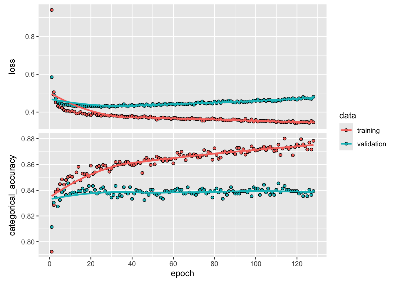
metrics <- model |>
      keras::evaluate(x = model_input$test$image,
                      y = model_input$test$label)
43/43 - 0s - loss: 0.8280 - categorical_accuracy: 0.7604 - 15ms/epoch - 342us/stepmetrics[1:2] loss categorical_accuracy
0.8280069 0.7603787 predicted_probs <- model |>
predict(model_input$test$image)43/43 - 0s - 33ms/epoch - 775us/stepdim(predicted_probs)[1] 1373 4predicted_probs[1:5,] [,1] [,2] [,3] [,4]
[1,] 0.9960365 0.003671102 0.0002693007 2.311535e-05
[2,] 0.9967024 0.003094842 0.0001937053 9.067555e-06
[3,] 0.9960365 0.003671102 0.0002693007 2.311535e-05
[4,] 0.9950758 0.004774944 0.0001432213 6.102709e-06
[5,] 0.9950406 0.004654717 0.0002965666 8.109485e-06test <- list(metrics = metrics,
year = cfg$train_test$test,
dates = model_input$test$dates,
locations = model_input$test$locations,
test_classifications = model_input$test$classifications,
test_toxicity = model_input$test$toxicity,
predicted_probs = predicted_probs)Using the model output, we can make a nice forecast table. In this example, we’re hindcasting so we will add the prediction and result to compare
f <- make_forecast_list(cfg, test)

glimpse(f)
Rows: 1,373
Columns: 13
Rowwise:
$ version <chr> "test", "test", "test", "test", "test", "test", "t…
$ location <chr> "PSP19.15", "PSP27.31", "PSP25.17", "PSP14.26", "P…
$ date <date> 2014-09-03, 2014-09-22, 2014-08-25, 2014-07-30, 2…
$ class_bins <chr> "0,10,30,80", "0,10,30,80", "0,10,30,80", "0,10,30…
$ forecast_start_date <date> 2014-09-07, 2014-09-26, 2014-08-29, 2014-08-03, 2…
$ forecast_end_date <date> 2014-09-13, 2014-10-02, 2014-09-04, 2014-08-09, 2…
$ actual_class <dbl> 0, 0, 0, 0, 0, 0, 1, 1, 0, 2, 1, 1, 2, 0, 0, 2, 0,…
$ actual_toxicity <dbl> 0.0000000, 0.0000000, 9.4264470, 0.0000000, 0.0000…
$ prob_0 <dbl> 99.603647, 99.670237, 99.603647, 99.507576, 99.504…
$ prob_1 <dbl> 0.36711020, 0.30948417, 0.36711020, 0.47749444, 0.…
$ prob_2 <dbl> 2.693007e-02, 1.937053e-02, 2.693007e-02, 1.432213…
$ prob_3 <dbl> 2.311535e-03, 9.067555e-04, 2.311535e-03, 6.102709…
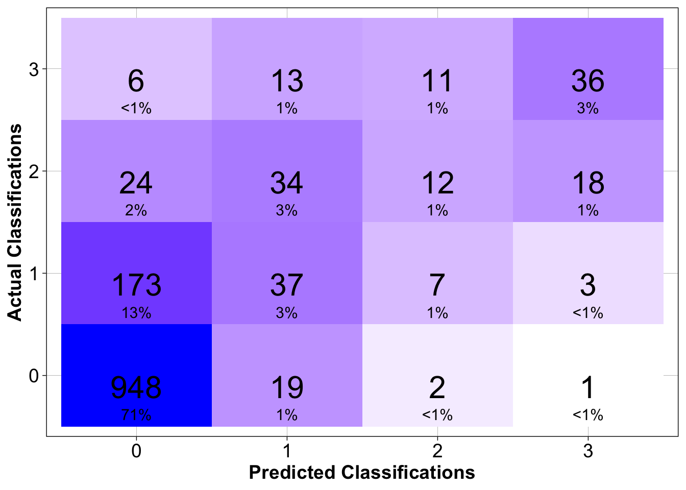
$ predicted_class <dbl> 0, 0, 0, 0, 0, 0, 0, 0, 0, 0, 0, 0, 2, 0, 0, 0, 0,…We can also use a confusion matrix to assess the skill of the model we built on a class-by-class basis
make_confusion_matrix(cfg, f)